
Lecture

Walsh functions are a family of functions that form an orthogonal system and take only the values +1 and −1 over their entire domain.
In principle, Walsh functions can be represented in continuous form, but more often they are defined as discrete sequences of  elements. A group of Walsh functions forms a Hadamard matrix.
Walsh functions have become widespread in radio communications, where they are used for code-division multiple access (CDMA), for example in cellular standards such as IS-95, CDMA2000 or UMTS.
The system of Walsh functions is an orthonormal basis and, as a consequence, makes it possible to expand signals of arbitrary shape into a generalized Fourier series.
A generalization of Walsh functions to the case of more than two values is the Vilenkin–Chrestenson functions.
Let a Walsh function be defined on the interval [0, T]; outside this interval the function repeats periodically. Introduce the dimensionless time  . Then the Walsh function with number k is denoted as
  . The numbering of the functions depends on the method of ordering them. There is Walsh ordering — in this case the functions are denoted as described above. Paley ordering (
 ) and Hadamard ordering (
  ) are also common.
With respect to the point  , Walsh functions can be divided into even and odd ones. They are denoted as
  and
and  respectively. These functions are analogous to the trigonometric cosines and sines. The relationship between these functions is expressed as follows:


There are several ways to construct them. Let us consider the most illustrative one: a Hadamard matrix can be built recursively by constructing block matrices according to the following general formula:
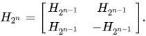
In this way a Hadamard matrix of length can be constructed:

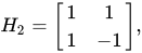
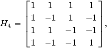
Each row of a Hadamard matrix is a Walsh function.
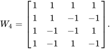
In this case the functions are in Hadamard order. The Walsh index of a function is computed from its Hadamard index by reversing the bits of the binary representation of the index and then converting the result from Gray code.
| Hadamard index | Binary form | Bit reversal | Conversion from Gray code | Walsh index |
|---|---|---|---|---|
| 0 | 00 | 00 | 00 | 0 |
| 1 | 01 | 10 | 11 | 3 |
| 2 | 10 | 01 | 01 | 1 |
| 3 | 11 | 11 | 10 | 2 |
The result is a Walsh matrix in which the functions are in Walsh order:
The inner product of two different Walsh functions is zero:
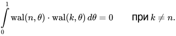
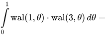
Suppose that n = 1, k = 3 (see above). Then

The product of two Walsh functions is a Walsh function:

where  denotes modulo-2 addition of the indices in binary form.
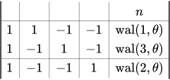
Suppose that n = 1, k = 3. Then

Multiplying, we obtain:
This is a special case of the generalized Fourier transform in which the basis is the system of Walsh functions.
A generalized Fourier series is represented by the formula
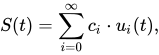
where  is one of the basis functions and
  is a coefficient.
The expansion of a signal in Walsh functions has the form
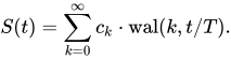
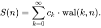
In discrete form the formula is written as follows:
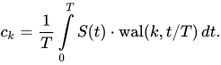
The coefficients can be determined by taking the inner product of the signal being expanded with the corresponding Walsh basis function:
The periodic nature of Walsh functions must be taken into account.
There is also a fast Walsh transform . It is considerably more efficient than the Walsh–Hadamard transform . In addition, for the special case of two variables, Walsh functions are generalized as surfaces . There are also eight bases of orthogonal binary functions analogous to Walsh functions , differing in their irregular structure, which are likewise generalized to the case of functions of two variables. For each of the eight bases, the representation of "step" functions as a finite sum of binary functions weighted with the corresponding coefficients has been proven .
The Walsh–Hadamard transform is a non-sinusoidal, orthogonal transformation method that decomposes a signal into a set of basis functions. These basis functions are Walsh functions, which are rectangular or square waves with values of +1 or –1. The Walsh–Hadamard transform is also known as the Hadamard (see the hadamard function in MATLAB software), Walsh, or Walsh–Fourier transform.
The first eight Walsh functions have these values:
| Index | Walsh function values |
|---|---|
| 0 | 1 1 1 1 1 1 1 1 |
| 1 | 1 1 1 1 -1 -1 -1 -1 |
| 2 | 1 1 -1 -1 -1 -1 1 1 |
| 3 | 1 1 -1 -1 1 1 -1 -1 |
| 4 | 1 -1 -1 1 1 -1 -1 1 |
| 5 | 1 -1 -1 1 -1 1 1 -1 |
| 6 | 1 -1 1 -1 -1 1 -1 1 |
| 7 | 1 -1 1 -1 1 -1 1 -1 |
The Walsh–Hadamard transform returns sequency values. Sequency is a more generalized notion of frequency and is defined as one half of the average number of zero crossings per unit time interval. Each Walsh function has a unique sequency value. You can use the returned sequency values to estimate the signal frequencies in the original signal.
Three different orderings are used to store Walsh functions: sequency, Hadamard, and dyadic. The sequency ordering, which is used in signal processing applications, places the Walsh functions in the order shown in the table above. The Hadamard ordering, which is used in control applications, arranges them as 0, 4, 6, 2, 3, 7, 5, 1. The dyadic or Gray code ordering, which is used in mathematics, arranges them as 0, 1, 3, 2, 6, 7, 5, 4.
The Walsh–Hadamard transform is used in many applications, such as image processing, speech processing, filtering, and power spectrum analysis. It is very useful for reducing storage and bandwidth requirements and for spread-spectrum analysis. Like the FFT, the Walsh–Hadamard transform has a fast version, the fast Walsh–Hadamard transform (fwht). Compared to the FFT, the FWHT requires less storage space and is faster to compute, because it uses only real additions and subtractions, while the FFT requires complex numbers. The FWHT can represent signals with sharp discontinuities more accurately using fewer coefficients than the FFT. Both the FWHT and the inverse FWHT (ifwht) are symmetric and thus use identical computation procedures. The FWHT and IFWHT for a signal x (t) of length N are given by:
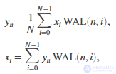
where i = 0,1, …, N – 1 and WAL (n, i) are the Walsh functions. Similar to the Cooley–Tukey algorithm for the FFT, the N elements are decomposed into two sets of N/2 elements, which are then combined using a butterfly structure to form the FWHT. For images, where the input is usually a 2D signal, the FWHT coefficients are computed by first evaluating across the rows and then down the columns.
For the following simple signal, the resulting FWHT shows that x was created using Walsh functions with sequency values 0, 1, 3, and 6, which are the nonzero indices of the transformed x. The inverse FWHT recreates the original signal.

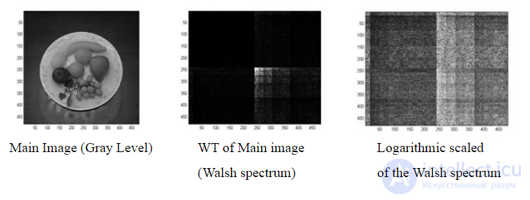
Walsh transform

Comments