
Lecture
Demand for a given good reflects the direct desire to buy that good and to pay a certain price for it. The volume of demand for a good is the quantity of that good that a single person or a group of persons is willing to buy per unit of time under given conditions. These conditions include the tastes and preferences of buyers, the prices of this good and of other goods, and the level of monetary income and savings.
Demand — is a request by an actual or potential buyer, a consumer, to acquire a good using the funds available to him that are intended for this purchase. Demand reflects, on the one hand, the buyer's need for certain goods or services, the desire to acquire these goods or services in a certain quantity, and, on the other hand, the ability to pay for the purchase at a price falling within the «affordable» range.
Supply — is the ability and willingness of a seller (producer) to offer goods for sale on the market at certain prices. This definition describes supply and reflects its essence from a qualitative standpoint. Quantitatively, supply is characterized by its magnitude and volume. The volume, or magnitude, of supply is the quantity of a product (good, service) that a seller (producer) wants, is able and is capable, in accordance with available resources or production capacity, of offering for sale on the market over a given period of time at a certain price.
The theory of demand and supply is a fundamental concept in economics that explains how prices and quantities of goods are formed on the market. This theory describes the interaction between buyers (demand) and sellers (supply) on the market, as well as the effect of prices on the quantity of goods that is bought and sold.
The law of demand: The law of demand states that, all else equal, the quantity of a good that consumers are willing to buy increases as the price of that good falls and decreases as it rises. In other words, there is an inverse relationship between the price of a good and demand for it: at lower prices consumers are willing to buy more, and at higher prices - less.
The law of supply: The law of supply states that, all else equal, the quantity of a good that sellers are willing to put on the market increases as the price of that good rises and decreases as it falls. That is, there is a direct relationship between the price of a good and its supply: at higher prices sellers are willing to offer more of the good, and at lower prices - less.
The interaction of the law of demand and the law of supply determines the equilibrium price and quantity on the market, which are called the equilibrium price and the equilibrium quantity. This is the price at which the quantity that buyers are willing to purchase coincides with the quantity that sellers are willing to offer.
If the price is above the equilibrium level, demand decreases and supply increases, which can lead to a surplus of the good. If the price is below the equilibrium level, demand increases and supply decreases, which can lead to a shortage of the good.
Thus, the theory of demand and supply helps explain how prices and quantities of goods are regulated on the market depending on the dynamics of demand and supply.
Like the volume of demand, the magnitude of supply depends not only on price but also on a number of non-price factors, including production capacity (see the Production Possibility Frontier), the state of technology, resource availability, the price level of other goods, and inflationary expectations.
Along with these general definitions, demand is characterized by a number of properties and quantitative parameters, among which the volume or magnitude of demand should above all be singled out.
From the standpoint of quantitative measurement, demand for a good, understood as the volume of demand, means the quantity of a given good that buyers (consumers) wish, are willing, and have the monetary means to purchase over a certain period within a certain price range.
The quantity demanded — is the amount of a good or service of a certain kind and quality that a buyer wishes to buy at a certain price over a certain period. The quantity demanded depends on buyers' incomes, the prices of goods and services, the prices of substitute goods and complementary goods, buyers' expectations, and their tastes and preferences.
Non-price characteristics of a good
But besides price, the quantity demanded is also affected by a number of other factors, sometimes called non-price factors. These are, above all, consumer tastes, fashion, the level of income (purchasing power), the level of prices of other goods, and the possibility of substituting the given good with others.
The demand price is the maximum price that buyers are willing to pay for a certain quantity of a given good. The dependence of the volume of demand on the factors determining it is called the demand function.
The inverse relationship between price and the volume of demand is called the law of demand.
However, one exception to this law is known, called the Giffen paradox or Giffen goods. This paradox consists in the fact that if a given good forms the basis of consumption, then even as its price rises, the volume of demand for it will increase. This paradox is the only exception to the law of demand, although there are other phenomena mistakenly taken for exceptions (price as an indicator of quality, the Veblen effect, the effect of expected price dynamics, or the Pigou effect).
Supply characterizes a seller's readiness to sell a certain quantity of a given good over a certain period of time. The volume of supply is the quantity of some good that a single seller or a group of sellers wishes to sell per unit of time under given conditions. These conditions include the nature of the technology used, the prices of this good and of other goods, including the prices of production resources (domestic and foreign), the presence and size of taxes and subsidies, as well as natural and climatic conditions. The supply price is the minimum price at which a seller is willing to sell a certain quantity of a given good. The dependence of the volume of supply on the factors determining it is called the supply function. Unlike the demand curve, the supply curve has a positive slope: as the price rises, the volume of supply also increases. However, this is not always the case, so unlike the general law of demand, which practically knows no exceptions, no such general law of supply exists. This positive slope of the supply curve is for now accepted as an assumption. As with demand, a distinction should be drawn between a change in the volume of supply and a change in supply. A change in the volume of supply occurs when the price of a good changes while the nature of the dependence of the volume of supply on price remains unchanged - a movement along the supply curve. But if, owing to a change in some non-price factor, a new relationship is established between price and the volume of supply, i.e. the supply function itself changes, then the supply curve shifts, and thus we are talking about a change in supply itself.
To examine the interaction of demand and supply, the demand and supply curves must be combined on a single graph. The abscissas of their points characterize, respectively, the volumes of demand and the volumes of supply, while the ordinates represent the demand prices and the supply prices. Market equilibrium is determined by the coordinates of the point of intersection of the demand and supply curves, to which the equilibrium volume and the equilibrium price correspond. In a state of equilibrium the market is balanced, and neither sellers nor buyers have any internal incentive to disturb it. However, at any price other than the equilibrium price the market is unbalanced, and buyers and sellers have effective incentives to change the situation that has arisen. At a price above equilibrium, a surplus of supply will exert downward pressure on the price. If, on the other hand, the actual price is below equilibrium, a shortage of supply (excess demand) will exert upward pressure on the price. In the first case this pressure is exerted through competition among sellers, and in the second - through competition among buyers. Note that one and the same person may act as both a buyer and a seller. This approach to describing equilibrium is called Walrasian equilibrium.
There is also an alternative approach, known as Marshallian equilibrium. Its essence is that equilibrium in the market is formed not under the influence of pressure from surpluses of demand and supply, but under the influence of the demand price exceeding the supply price, or vice versa, to which sellers respond by correspondingly increasing or reducing the volume of supply. If the volume of supply is below the equilibrium level, the demand price is higher than the supply price, which induces sellers to increase the volume of supply. If the volume of supply exceeds the equilibrium level, the supply price is higher than the demand price, which induces sellers to reduce the volume of supply. The difference between these approaches is also reflected in the different arrangement of the coordinate axes on the demand and supply graphs. Marshall operated with the concepts of demand price and supply price, so for him the demand and supply function takes the form P= P(Q). And the equilibrium condition is Pd(Q)=Ps(Q). The volumes of demand and supply, as the independent variables, were plotted on the abscissa axis.
Walras, on the other hand, focused attention on the volumes of demand and supply at given prices. Therefore his demand and supply function takes the following form. Q=Q(P). Then equilibrium is reached when Qd(P)=Qs(P).
Modern economic theory works with demand and supply functions in the Walrasian manner, and with graphical representation in the Marshallian manner.
Static models do not take the time factor into account. The comparison of instantaneous states of dynamic processes is called the method of comparative statics. In this approach, different equilibrium states of the market are compared without considering the actual process of transition from one state to another. Although the method of comparative statics does not explicitly take the time factor into account, its indirect inclusion becomes possible through allowing for differences in the speed at which supply adjusts to changes in demand. For this purpose, when using the method of comparative statics, it is customary to distinguish three periods. The first, in which all factors of production are treated as fixed, is called the momentary period. Another, in which one group of factors is treated as fixed and another as variable, is called the short period. The third, in which all factors of production are treated as variable, is called the long period. One may further distinguish a fourth, very long period, during which not only the volume of resources used and the intensity of their use may change, but also the nature of the technology employed.
In the momentary period the seller is unable to adjust the volume of supply to the volume of demand, since the quantity of production resources and the intensity of their use are fixed. However, this given quantity of the good may be sold at different price levels. Much also depends on the nature of the good itself. If the good is not storable, the supply curve will be vertical to the abscissa axis. In this case the equilibrium price is determined by demand and coincides with the demand price, while the volume of supply is fixed.
If the good is not perishable, the supply curve may be represented as consisting of two segments: one having a positive slope, and a second representing a vertical segment. In this case, at a price below Pe the seller will offer not the entire good but only part of it, since part of the good can be held in storage until more favorable market conditions arise.
If, however, storing the surplus is difficult or involves high costs, the corresponding quantity of the good may be sold off at give-away prices.
Over the course of the short period the firm's production capacity is considered unchanged, but its utilization and the volume of output can change owing to changes in the amount of variable factors employed.
These changes cannot go beyond the limits of the technical production capacity. In the short period the supply curve likewise consists of two segments. The first has a positive slope. The second segment of the supply curve is represented by a vertical segment, which indicates the impossibility, within the short period, of going beyond the limits set by the available production capacity. Up to this boundary, the equilibrium volume and price are determined by the intersection of the demand and supply curves, while beyond it, as in the momentary period, the price is determined by demand, while the volume of supply is determined by the size of production capacity.
In the long period the producer can not only vary the intensity with which production capacity is used, but also change its size, and hence the scale of production. In the long period three situations are possible: first, when costs remain constant, in which case the equilibrium price does not change; second, with rising costs, in which case the equilibrium price rises together with the increase in the volume of supply; and third, with falling costs, in which case the supply curve has a negative slope and an increase in the volume of supply is accompanied by a fall in the equilibrium price.
The supply curve can change its slope, which ultimately leads to non-uniqueness of the equilibrium state. A characteristic example of a situation of non-unique equilibrium is provided by the illustration of equilibrium in an individual labor market.
Stability of equilibrium is the name given to the ability of a market that has been driven out of a state of equilibrium to return to equilibrium under the influence of its own internal forces alone. The problem of stability has significance beyond the purely economic, since the possibility of state regulation of the market, in cases where it is incapable of self-regulation, ensures the maximum welfare and social security of the population.
If the demand curve and the supply curve have the normal slope (positive and negative, respectively), the equilibrium is stable. The interaction of demand and supply, both in the Walrasian sense and in the Marshallian sense, will bring the market to a state of equilibrium. It is a different matter if the supply curve has a negative slope; in this case, the market's ability to move out of a state of disequilibrium depends on which principle governs the interaction - the Walrasian or the Marshallian.
The direct price elasticity of demand characterizes the relative change in demand for a good in response to a change in its price. The coefficient of direct price elasticity of demand is the ratio of the relative change in the volume of demand, in percent, to the relative change in price:
A distinction is drawn between point elasticity and arc elasticity. Point elasticity (or elasticity at a point) characterizes the relative change in the volume of demand for an infinitesimally small change in price.
The direct price elasticity of demand depends on the availability of substitute goods, on the variety of possible uses of the given good, on the degree to which needs are satisfied, and on the time factor. Demand is more elastic in the long period than in the short period, since time is needed to adjust to changed prices.
The cross-price elasticity of demand characterizes the relative change in the volume of demand for one good in response to a change in the price of another. The coefficient of cross-price elasticity of demand is the ratio of the relative change in demand for good i to the relative change in the price of good j.
The cross-elasticity coefficient may be positive, negative, or zero.
The main factor determining the cross-price elasticity of demand is the natural properties of goods, their capacity to substitute for one another in consumption.
The income elasticity of demand characterizes the relative change in demand for a given good as a result of a change in the consumer's income. The coefficient of income elasticity of demand is the ratio of the relative change in the volume of demand for good i to the relative change in the consumer's income:
The concept of elasticity extends not only to such an economic category as demand - it can also be used to determine how the quantity supplied reacts to price changes. Formally, the coefficient of price elasticity of supply has the same form as the coefficient of direct price elasticity of demand. Only its economic meaning consists in the fact that it shows the percentage change in the quantity of a good supplied relative to the percentage change in the price of that good. The methods for calculating the coefficient of elasticity of supply fully coincide with the analogous methods for the coefficient of elasticity of demand.
The main factors determining the elasticity of supply are, first, the mobility of factors of production. Second, there is the time factor. As with demand, the price elasticity of supply tends to increase over longer time intervals. Over time, producers' adaptation to new market conditions improves the market opportunities for matching their output to the increased demand, which leads to an increase in the elasticity of supply.
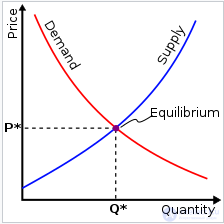
The law of supply and demand — an economic law combining the law of demand and the law of supply. Usually the price is set at the point of equilibrium between supply and demand. Other things being equal, a decrease in the price of a good increases demand (willingness to buy) and decreases supply (willingness to sell).
The law of demand — the quantity (volume) of demand decreases as the price of a good increases. Mathematically, this means that there is an inverse relationship between the quantity demanded and the price (though not necessarily in the form of a hyperbola represented by the formula y = a/x). That is, a rise in price causes a decrease in the quantity demanded, while a decrease in price causes an increase in the quantity demanded.
The nature of the law of demand is not complicated. If a buyer has a certain amount of money to purchase a given good, he will be able to buy less of the good the higher the price, and vice versa. Of course, the real picture is much more complex, since the buyer can raise additional funds or buy another good instead of the given one — a substitute good.
Non-price factors affecting demand:
In a number of microeconomics courses the law of demand is formulated more strictly: If, as income rises, demand for a good increases, then as the price of that good rises, demand for it must decrease.
This correction is due to the existence of Giffen goods, for which the quantity demanded rises as the price rises. But for the overwhelming majority of cases (given the rarity of Giffen goods) the above pattern holds.
The elasticity of demand is an indicator expressing the fluctuations in aggregate demand caused by changes in the prices of goods and services. Demand is called elastic if it forms under the condition that the change in its volume (in %) exceeds the percentage decrease in prices.
If the percentage figures for the fall in prices and the increase in demand are equal, that is, the growth in the volume of demand merely compensates for the decline in the price level, then the elasticity of demand is equal to one.
In the case where the degree of the price decrease exceeds the demand indicator for goods and services, demand is inelastic. Consequently, the elasticity of demand is an indicator of the degree of sensitivity (reaction) of consumers to changes in the price of a good.
The elasticity of demand may be related not only to a change in the price of a good but also to a change in consumers' incomes. Therefore a distinction is made between price elasticity of demand and income elasticity of demand. There is also demand with unit elasticity. This is a situation in which both income and the quantity demanded change by the same percentage, so that total revenue remains constant as the price changes.
The reaction of consumers to a change in the price of a good can be strong, weak, or neutral. Each of these gives rise to a corresponding type of demand: elastic, inelastic, unitary. There are also cases in which demand turns out to be perfectly elastic or perfectly inelastic.
The elasticity of demand is measured quantitatively through the elasticity coefficient using the formula:

As a rule, goods exist with different price elasticities. In particular, bread and salt are examples of inelastic demand. A rise or fall in their prices generally does not affect the quantity consumed.
Knowledge of the degree of elasticity of demand for a good has great practical significance. For example, sellers of a good with high demand elasticity may resort to lowering the price in order to sharply increase sales volume and obtain more profit than if the price of the good were higher.
For goods with low demand elasticity, such a pricing practice is unacceptable — when the price is lowered, the sales volume will change only slightly and will not compensate for the lost profit.
When there is a large number of sellers, demand for any good will be elastic, since even a slight increase in price by one of the competitors will force consumers to turn to other sellers offering the same good more cheaply.
The demand curve shows the probable quantity of a good that can be sold in a given period of time at a given price. The more elastic the demand, the higher the price that can be set for the good. The elasticity of demand is the market's reaction to the absence of a good, the possibility of replacing it, competitors' prices, price reductions, buyers' reluctance to change their consumption habits and look for cheaper goods, improvements in the quality of goods, and the natural growth of inflation relative to other factors.
All producers (sellers) in the market are united by supply: at a low price the seller will offer less of the good or may hold it back; at a high price he will offer more of the good; at a very high price he will try to increase production as much as possible. In this way the supply price is formed — the minimum price at which sellers are willing to sell their goods…
The law of supply — other factors being unchanged, the quantity (volume) of supply increases as the price of a good increases.
The growth in the quantity supplied of a good as its price rises is, in general, due to the fact that with unchanged costs per unit of the good, profit rises as the price rises, and it becomes profitable for the producer (seller) to sell more of the good. The real picture in the market is more complex than this simple scheme, but the tendency expressed in it does hold.
Factors affecting supply:
The elasticity of supply — an indicator reflecting the changes in aggregate supply that occur in connection with rising prices. In the case where the increase in supply exceeds the increase in prices, the latter is characterized as elastic (the elasticity of supply is greater than one — E> 1). If the increase in supply equals the increase in prices, the supply is called unitary, and the elasticity indicator is equal to one (E = 1). When the increase in supply is less than the increase in prices, so-called inelastic supply is formed (the elasticity of supply is less than one — E <1). Thus, the elasticity of supply characterizes the sensitivity (reaction) of the supply of goods to changes in their prices.
The elasticity of supply is calculated using the elasticity coefficient of supply by the formula:

The elasticity of supply depends on such factors as the characteristics of the production process, the time it takes to manufacture the product, and its capacity for long-term storage. The characteristics of the production process allow the producer to expand production of a good when its price rises, while when its price falls the producer switches to manufacturing other products. The supply of such a good is elastic.
The elasticity of supply also depends on the time factor, when the producer is unable to react quickly to price changes because additional production of the good requires a significant amount of time. For example, it is practically impossible to increase automobile production within a week, even though their price may rise many times over. In such cases supply is inelastic. For a good that cannot be stored for a long time (for example, products that spoil quickly), the elasticity of supply will be low.
Many economists identify the following factors that change supply:
The supply curve shows the relationship between market prices and the quantity of goods that producers are willing to offer.
The main factor affecting the movement of the supply curve is the cost of production. As is well known, firms manufacture goods for the sake of profit. For example, farms grow wheat. They grow more wheat because at the given moment it is more profitable to sell wheat than another crop. And vice versa.
The second factor affecting the movement of the supply curve is technical progress. New seed stock, a more efficient tractor, a better crop-rotation computer program — all of this allows the farmer to reduce production costs and change the supply of his product. Production costs are a key element of the long-term effect on the «supply curve».
The Arab Muslim philosopher, historian, and social thinker Ibn Khaldun postulated in the 14th century that the price of goods and services is determined by supply and demand. If a good is scarce and in demand, its price is high, and if there is a lot of the good and it is not in demand, its price will be low. An entrepreneur pursuing profit will buy a good where it is cheaper and not in short supply, and sell it where it is in demand, at a higher price.
The first detailed elaboration of the law of supply and demand appeared in the works of the Spanish and Peruvian jurist and economist Juan de Matienzo in the second third of the 16th century.
His theory of subjective value leads to a distinction between the elements of demand and supply within the market. Matienzo uses the term «competition» to describe rivalry within a free market. This served as the basis for defining the concepts of public auctions and the rivalry between buyers and sellers.
In addition to supply and demand, Matienzo also considered other factors affecting the determination of a just price, describing the highly variable morphology of the market. In the posthumously published treatise «Commentaria Ioannis Matienzo Regii senatoris in cancellaria Argentina Regni Peru in librum quintum recollectionis legum Hispaniae. — Mantuae Carpentanae : Excudebat Franciscus Sanctius, 1580» the following are listed:
A market economy can be viewed as an endless interaction of supply and demand, where supply reflects the quantity of goods that sellers are willing to offer for sale at a given price at a given time. The law of supply is an economic law according to which the quantity of a good supplied in the market increases as its price rises, other things being equal (production costs, inflation expectations, the quality of the good). In essence, the law of supply says that at high prices more goods are offered than at low prices. If supply is represented as a function of price in terms of the quantity of the good offered, the law of supply describes the increasing nature of the supply function over its entire domain. Similarly, the law of demand means that at a low price buyers are willing to purchase more of a good than at a high price. The demand function, as a function of price in terms of the quantity of the good purchased, is decreasing over its entire domain.
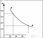
The law of demand
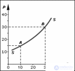
The law of supply
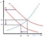
Change in demand occurs under the influence of the determinants of demand, while supply remains unchanged, other things being equal. A rightward shift of the demand curve increases demand, leading to a new equilibrium state in which the intersection point of the supply and demand curves is higher than the previous state, as shown in the graph Increase in demand. A price-increase effect and a quantity-increase effect are observed. In the graph Decrease in demand, where the demand curve shifts to the left, the new equilibrium point is lower than the previous state. A price-decrease effect and a quantity-decrease effect are observed. From this it is concluded that there is a direct relationship between a change in demand and changes in the equilibrium price and quantity of the product .
Change in supply occurs under the influence of the determinants of supply, while demand remains unchanged, other things being equal. A rightward shift of the supply curve increases supply, leading to a new equilibrium state in which the intersection point of the supply and demand curves is lower than the previous state, as shown in the graph Increase in supply. A price-decrease effect and a quantity-increase effect are observed. In the graph Decrease in supply, where the supply curve shifts to the left, the new equilibrium point is higher than the previous state. A price-increase effect and a quantity-decrease effect are observed. From this it is concluded that there is an inverse relationship between a change in supply and changes in the equilibrium price and quantity of the product .
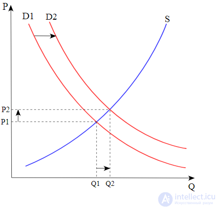
Increase in demand
Decrease in demand
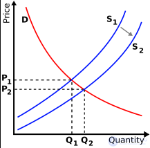
Increase in supply
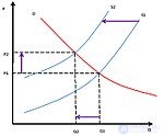
Decrease in supply

Comments