
Lecture
Theory of Market Organization (TOM)– is largely a central subject in economics, or at least in microeconomics. How do firms compete? What strategies do firms have for competing «better»? When is it more profitable for firms to act aggressively, and when is it not? The answers to these and similar questions are important for understanding the behavior of firms in practice and the functioning of real markets
The model of the perfectly competitive market is based on the assumption that, within its framework, there is no competition between sellers and buyers in the traditional sense of the word. Perfect competition is perfect in the sense that each firm can sell as much output as it wishes at the given market price, and the price level cannot be influenced by any individual seller or any individual buyer. The model of perfect competition is based on several assumptions.
- homogeneity of output. This means that all units of output are completely identical and buyers have no way to distinguish by whom exactly one unit or another was produced. The set of all firms producing a homogeneous product forms an industry. Thus, it can be noted that the anonymity of sellers together with the anonymity of buyers makes the perfectly competitive market completely impersonal.
- smallness and multiplicity. This means that the smallness of market participants means that the volumes of demand and supply are negligibly small relative to the scale of the market. The smallness and multiplicity of market participants presupposes the absence of formal or informal agreements between them aimed at obtaining monopoly advantages. The assumptions of product homogeneity, multiplicity, and their smallness form the basis for the following important assumption. Under perfect competition, each individual producer is a price taker: that is, the demand curve for its output is infinitely elastic and has the form of a straight line parallel to the abscissa axis, and the seller can sell any volume of output at the prevailing market price. Since in this case total revenue TR grows in proportion to the increase in output, average and marginal revenue from its sale are equal and coincide with the price (P=AR=TR). That is why the demand curve in the model of perfect
competition is at the same time the line of average and marginal revenue.
- freedom of entry and exit. All sellers and buyers have complete freedom to enter the industry and exit it. Likewise, buyers are free to purchase the good in any quantity and to stop purchasing it. There are no legal or financial barriers to entry into the industry. Freedom of entry and exit for sellers and buyers also presupposes perfect mobility of buyers and sellers within the market, and the absence of any forms of attachment of buyers to sellers.
- perfect information. Market participants possess perfect knowledge of all market parameters. Information spreads among them instantly and costs them nothing.
Under perfect competition, a firm is a price taker. It can maximize its profit only by adapting the volume of output to the conditions of the product market, on the one hand, and, on the other, to its own costs determined by technology. But it cannot influence the price.
There are two main approaches to determining the level of output at which a firm will earn maximum profit. The first involves comparing total revenue and total costs, the second, marginal revenue and marginal costs.
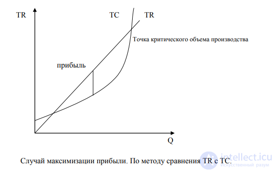
The case of profit maximization. Using the method of comparing TR and TC.
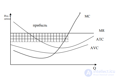
The case of profit maximization using the method of comparing marginal revenue with marginal
cost. The firm maximizes profit if MC exceeds both total and average
cost. If you look carefully at the marginal cost graph, you can
notice that the firm will produce output starting from the point where the
marginal cost curve intersects the average variable cost curve, at the corresponding
market price. Thus, the segment of the firm's marginal cost curve that
lies above its average variable cost curve is the supply curve in
the short run.
If an unfavorable price for obtaining maximum profit develops in the market, then
the firm can minimize its losses either by remaining in the industry and producing
further output, or by shutting the firm down entirely. Using the first method, the firm
will minimize its losses by producing such a volume of output at which
total costs exceed total revenue by the minimum amount. However, if
there is no output level at which total revenue exceeds variable costs, the firm
will minimize its losses in the short run by shutting down.
Using the second approach, if the price exceeds the minimum of AVC, but
is less than ATC, the firm minimizes its loss by remaining in the industry. If the price
falls below the minimum of AVC, the competitive firm will minimize its
losses by shutting down. There is no level of output at which the firm can
produce and incur a loss smaller than its fixed costs.
What we examined earlier concerned the demand and supply curves of an individual firm
or enterprise. However, as stated above, in the model of perfect competition
entire industries exist that produce a homogeneous product. The demand curve of an individual
firm, as already mentioned, is represented by a horizontal line that coincides with
MR and P. The industry demand curve represents the sum of the demand curves of individual firms and
has the usual negative slope. The same applies to industry supply,
which is also formed as the sum of the supply curves of individual firms.
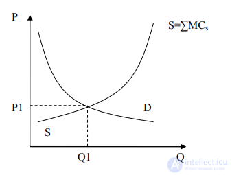
The price of the product is a given quantity for an individual firm, while at the same time the plans
of the entire industry for producing this product are a factor in price changes.
Although each individual firm cannot influence the price, the sum of the supply curves of the entire
set of firms in the industry makes up the industry supply curve. Thus, under
conditions of competition, the equilibrium price is a given quantity for the individual
firm, and at the same time is the result of the production decisions of all firms, taken as a
group.
The long run allows firms to make certain changes. Thus, in
this period firms can reduce or expand their production capacity, and
the number of firms in the industry itself can also increase or decrease. Let us consider
how long-run equilibrium will be established in the industry.
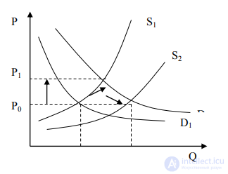
A favorable shift in demand to D2 will disturb the initial equilibrium and give rise to
economic profits. But the profits will induce new firms to enter the industry, increasing
supply to S2 and lowering the price of the product, until economic profits once again
become zero. Thus, after adjustment to long-run equilibrium
the price of the product will correspond exactly to the minimum point of average
total cost, and output will fall at the same point. This conclusion follows from two
basic facts: 1) firms strive for profits and avoid losses; 2) under
competition firms freely enter and leave the industry, which leads to a change
in price for a short period, and then returns it to its original state.
Now let us consider supply in the long run. In the long run, all
industries were considered as groups with constant costs. This means that
the expansion of the industry through the entry of new firms will not affect the prices
of resources or, consequently, the costs of production. Thus, it can be said
that in the long run the supply curve of a constant-cost industry
will be perfectly elastic.
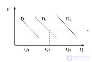
Since the entry or mass exit of firms does not affect resource prices,
or the cost per unit of output, an increase in demand will cause an expansion
of industry output, but no change in price will occur. The same applies
to a decrease in demand.
However, constant-cost industries are quite rare. Most industries
are increasing-cost industries, and their average cost curves shift upward as the industry expands, and downward when the industry contracts.
When an industry uses a significant share of some resource, the total volume
of supply of which is not easy to increase, the entry of new firms will increase
demand for the resource and raise its price. This is exactly what happens in industries where
highly specialized resources are used, whose initial supply
cannot be quickly increased. The result of higher resource prices
will be higher average costs for firms in the industry in the long run.
An outstanding contribution to the analysis of the imperfectly competitive market was made by such
economists as Antoine Cournot, Edward Chamberlin, J. Robinson, J. Hicks, and others. The market
of imperfect competition is represented by such market models as monopoly (a single
seller), monopsony (a single buyer), monopolistic competition, oligopoly,
and duopoly. In real life, pure monopoly does not exist; this can
only be spoken of with a degree of convention, since there is no firm
producing output that has no substitutes. Perfect competition and
pure monopoly – are theoretical abstractions that express two polar
situations in the market.
The model of monopoly is based on the following assumptions:
The main difference in the behavior of a perfectly competitive firm and
a monopolist is due to the different nature of their demand curves. A perfectly competitive
firm can sell as much as it wants without affecting the market price,
hence the demand curve is represented by a horizontal line. In the case of an imperfectly competitive firm, the demand curve has a negative slope, because the
larger its output, the lower the price it can set. Consequently, when a monopolist firm puts a larger quantity of the good on the market, its price falls. This
circumstance also affects the shape of the marginal revenue curve MR. Under
perfect competition MR=D=AR=P. Under pure monopoly, however, the
marginal revenue line lies below the price, i.e., MR<P. This is because, in order to sell
an additional unit of output, the imperfect competitor lowers the price. This
reduction gives it a certain gain, but at the same time it also brings certain
losses. The point is that, by lowering the price, for example on the third unit of the good, it thereby
effectively lowers the price of the preceding units as well; now all buyers pay less,
including those who could have paid the old price, and this loss is subtracted from the price,
which lowers marginal revenue.
In addition, the total revenue curve also has a special shape. To sell
an additional quantity of output, the monopolist must lower the price; this
reduction is offset, up to a certain point, by an increase in sales volume, but
only up to a certain limit; a further reduction in price will no longer lead to an increase in
revenue, which is why the total revenue graph has a hill-shaped form.
There is a special relationship between the MR and TR lines: moving down along
the elastic segment of the demand curve, TR increases, and consequently MR is
positive. When TR reaches its maximum, MR equals zero, and moving
down along the inelastic segment of the demand curve, TR decreases so that MR becomes
negative. A monopolist or other imperfect competitor will never want
to lower the price on the inelastic segment of the demand curve, because it would simultaneously
reduce total revenue and increase production costs, which lowers its
profit.
The monopolist will maximize profit by influencing either the volume of output or the
price, unlike a perfectly competitive seller, who regulated only
the volume of output. When comparing TR with TC, profit will be maximal at
the point of the greatest difference between these two quantities.
Under pure monopoly, the monopolist maximizes profit by producing a volume
of output at which MR=MC; in this case, profit per unit of
output is Pa, and total profit is the white rectangle. The point is that
the monopolist seeks not to maximize profit per unit of output, but to maximize
total profit. Thus, the graph shows that the point corresponding to Pa yields
more profit per unit, because it corresponds to a larger volume; however
the monopolist will stick to a smaller volume, because additional
sales compensate for the lower profit per unit.
Monopolistic competition implies a market situation in which
a relatively large number of small producers offer similar but
not identical products. The assumptions underlying the model of monopolistic
competition represent something of a mixture of the assumptions adopted for perfect
competition and monopoly.
A firm will maximize its profits or minimize its losses in
the short run by producing the volume of output determined by
the intersection of the marginal cost and marginal revenue curves. But a
less favorable situation with costs and demand may also arise, placing a firm operating under
monopolistic competition in a position where it incurs losses in
the short run. In the short run, a firm operating under conditions of
monopolistic competition may either earn economic profit or
face losses. In the long run, there is a tendency toward earning
normal profit.
Economic profits will induce new firms to enter the industry, and as a result, in the course of
competition they will be eliminated. Losses will cause a mass exodus of firms from the industry
until normal profits are restored. Thus, if the price merely
covers the cost per unit of output at the volume of production for which
MR=MC, a position of equilibrium is reached in the long run.
The word oligopoly is derived from Greek and was introduced into the English vocabulary by Thomas More. Today this word is used by economists as a term denoting a particular type of market structure in which the supply side is represented by a small number of relatively large firms – sellers of a homogeneous product or close substitutes. The distinctive feature of oligopoly lies in the universal interdependence of the conduct of the seller firms. An oligopolist firm cannot help but take into account that the relationship between the price level it chooses and the quantity of output it will be able to sell at that price depends on the behavior of its rivals, which in turn depends on the decision it makes. The model of oligopoly is based on the following assumptions: - output may be either homogeneous or differentiated; - a small number of sellers; the possibility of entry into the industry varies widely, from completely blocked entry to entirely free entry. The concentration of the market and the degree of power over price under oligopoly can be measured using the Herfindahl index (H). When calculating the Herfindahl-Hirschman index, market shares can be measured either as decimal fractions or as percentages. Its values lie between zero and one when calculated as decimal fractions, and between 1 and 10000 when calculated as percentages. Constructing this index requires a preliminary estimate of a firm's share of the market, that is, its share of the industry's total sales volume (in percent), denoted by the symbol S. For example, if one of the firms supplies 50% of the entire industry's sales volume to the market, then its S=50%. Next, it is necessary to determine how many firms there are in total in the industry (from 1 to n). Each firm's indicator is then squared and all the indicators are summed:
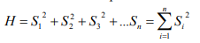
in the case of pure monopoly, the Herfindahl index will equal 10000; if there are two oligopolist firms in the industry, then H = 5000. In the case of perfect competition, the Herfindahl index equals 100.
Another index used to assess the degree of concentration and monopolization
is the elementary concentration ratio (CRk), which is calculated by
summing the market shares of the largest firms in the industry.
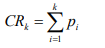
where pi=q1/Q denotes the share of output of the i–th producer (qi) in the total volume of
industry production
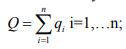 ; n – the total number of firms in the industry, k - the number of leading firms taken into account when calculating the index, usually equal to three, four,
six, or eight; the concentration index lies between zero and one and makes it possible to
determine the type of market structure in the sectors of the country's economy. The higher its
value, the stronger the tendency toward monopolization of the given industry, and the lower
the competitive advantages of outsider firms not taken into account when calculating this
index. For aggregated branches of Russian industry, the following
values of this index are typical. Four broad groups of market structures are distinguished:
pure monopoly pi=100%; a dominant firm or group of firms (50%<pi<90%);
restricted oligopoly with stable market shares (CRk<60%); and effective
competition, which includes expanded oligopoly, monopolistic competition, and
also perfect competition (CRk<40%).
There are a sufficient number of theories describing the behavior of an oligopolist in setting the maximum volume of output and maximum profit. Among the best known, one can note the duopoly theory of A. Cournot and E. Chamberlin. Let us now turn to the pricing of oligopoly that is not based on secret collusion. It is important to emphasize that in the case of oligopoly, competition is non-price in nature. Non-price competition is based on attracting the consumer not by lowering the price, but through other factors: improving the quality of goods, advertising, after-sales technical service, and so on. Each oligopolist takes into account that a reduction in its price will provoke a response from other oligopolists. Therefore
the demand that has increased owing to the lower price will be distributed among all the firms, and the firm that first lowered its price will receive only a portion of the increased demand. It is another matter if a firm raises its price; in this case the other oligopolists may not follow suit, and this is what usually happens, so demand for its product will fall considerably more sharply than would occur in the case of a general price increase.
The shape of the demand and marginal revenue curves of an oligopolist not participating in secret collusion will depend on whether its competitors match their prices to its prices (D1D1 and MR1MR1) or ignore any changes in the current price. Ignoring a price increase while following a price decrease results in a demand curve with a kinked shape (D2PD1), and the marginal revenue curve has a vertical gap. This gap arises because of the sharp differences in the elasticity of demand above and below the current price point. This model was proposed by the American economist Paul Sweezy.

Comments