The digital spectral analysis is based on the discrete Fourier transform (DFT) apparatus. In this case, the DFT has high-performance fast algorithms (FFT). However, when using the DFT, difficulties often arise due to the finiteness of the treatment interval. In this article we will set a goal to analyze the effects arising from the limitation of the analysis interval. It is assumed that the reader has previously studied the Fourier transform and its properties, and also understands the meaning of the DFT.
Spectrum of a time-limited signal
Let there be a signal

which is infinite in time. In the simplest case, we can define this signal as a harmonic oscillation with a frequency

. The Fourier transform of this signal will be a delta pulse at the signal frequency, i.e.
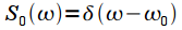
. The original signal and its spectrum are shown in blue in the figure. In practice, we cannot calculate the spectrum by numerical integration over the entire time axis (of course, except when we can obtain an analytical expression for the signal spectrum, as in the above example), so we fix the time interval

on which we will calculate the spectrum of the signal. This way we get the signal

that matches the original on the time interval
but outside the observation interval we consider

. Mathematically,
can be represented as a product of the original infinite signal

and square pulse

duration
,
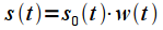
. Signal spectrum
, according to the properties of the Fourier transform will be equal to the convolution of the spectra of the original signal and the spectrum

square pulse
:
 |
(one) |
In expression (1), the filtering property of the delta function was used. Signal
and its spectrum

shown in Figure 1 in red.

Figure 1: Spectrum of a time-limited signal
Thus, instead of a delta pulse, the spectrum

turned into a type function

(spectrum of a square wave function
) and the width of the petal depends on the duration of the analysis interval, as is clearly shown in Figure 2.
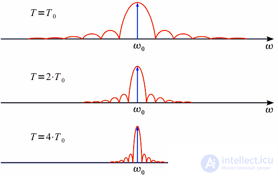
Figure 2: Spectrum changes with an increase in the analysis interval
If you increase the analysis interval

to infinity, the spectrum will narrow and strive for a delta pulse. Square pulse

let's call the window function.
DFT of a time-limited signal. Using window smoothing
Now consider the case of DFT. DFT sets in compliance

signal readings
spectrum readings taken on one repetition period of the spectrum:
Signal samples taken at regular intervals
Where

- sampling rate (rad / s). Thus, the analysis interval
then the spectral readings are taken at intervals
The width of the main lobe of the spectrum
(see picture 1) equals

then we can consider two cases. The first case is the frequency of the signal coincides with

frequency spectrum

(top graph of figure 3). When sampling, we only get the countdown at the frequency
the amplitude of the corresponding amplitude of the signal, the remaining spectral samples will be zero, since the spectral sampling times coincide with the zeros of the spectrum of the window function. The second case is when the frequency

does not coincide with any frequency from the grid of spectral samples (lower graph of figure 3). In this case, the spectrum of the signal "blurred." Instead of a single spectral sample, we get a set of samples, since the discretization is no longer done at the zeros of the spectrum of the window function, and all side lobes appear in the spectrum. In addition, the amplitude of the spectral samples also decreases.
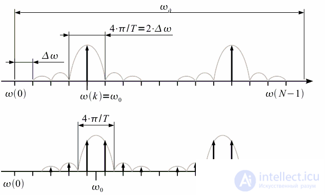
Figure 3: DFT with coincidence and mismatch of the signal frequency and spectrum frequency grid
The coincidence of the frequency with the grid of spectral samples will be in the case if the processing interval fits a whole number of periods of the signal. Otherwise, the spectrum will "smear."
Spectrum spreading is a negative effect that needs to be addressed. Let's show it by example. Let there be two harmonic signals at frequencies
and

, with the amplitude of the signal at the frequency
A lot less signal amplitude at frequency
. Limiting the analysis interval will cause the spectra to "smear" and the signal at the frequency
will not be noticeable under the side lobe signal with a frequency
as shown in Figure 4.
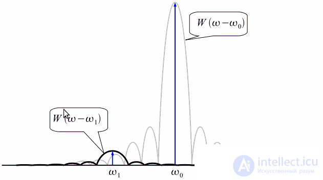
Figure 4: A small amplitude signal is not noticeable under the side lobe of another signal.
Obviously, in order to detect a weak signal, it is necessary to eliminate the side lobes in the spectrum that arise when we have limited the signal to a rectangular window. So in order to eliminate these petals it is necessary to eliminate them in the spectrum of the window function.
, that is, it is necessary to change the window function, namely to make it smoother, as shown in Figure 5.
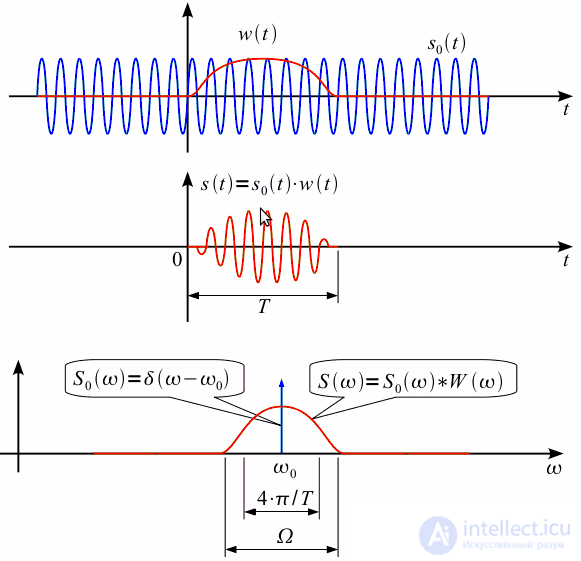
Figure 5: Smooth weight function
With a smooth window function, no side lobes are observed in the spectrum (or their level decreases significantly), however, there is an expansion of the main spectrum lobe compared to a rectangular window.
. Thus, we seem to have overcome the side lobes, and were able to detect weak signals (see Figure 6), which were previously lost in the side lobes, but paid for this by extending the main lobe.
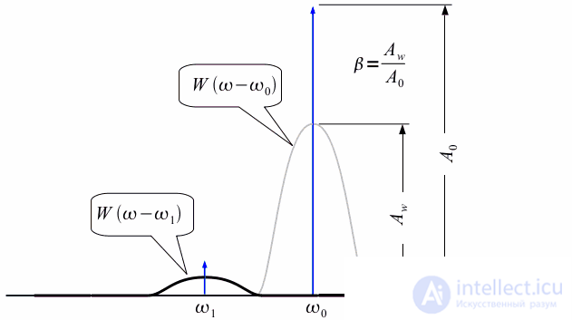
Figure 6: With a smooth weight function, weak signals are not lost in the side lobes
It should be noted that the greater the suppression of the side lobes of the spectrum of the window function, the wider the main lobe is obtained. This contradiction led to the development of a large number of window functions with different suppression of side lobes and different widths of the main lobe. The main common windows will be discussed below.
Window attenuation coefficient
We will consider another property of the window function, namely, the attenuation coefficient

. To clarify the attenuation coefficient
consider the constant component

window function on the interval
:
 |
(2) |
In the case of a rectangular window
 |
(3) |
Attenuation coefficient
called the ratio of the constant component
a given window function, to the constant component of a rectangular window

:
 |
(four) |
The meaning of the attenuation coefficient is that the amplitudes of all spectral components after multiplying by the window function decrease in
times compared to a rectangular window. The attenuation coefficient is expressed in a logarithmic scale:
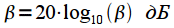 |
(five) |
In the case of digital spectral analysis there is

window function count
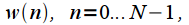
taken through the gap

Then

the integral in expression (4) is replaced by the sum:
 |
(6) |
In order to take into account the attenuation coefficient after the DFT, each spectral sample should be divided by
.
The main frequency characteristics of the spectrum window function
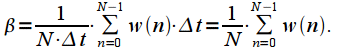
Let us generalize the main frequency characteristics of the spectrum of the window function, allowing to compare different windows with each other. To do this, consider the normalized amplitude-frequency characteristic

window function shown in Figure 7.
Figure 7: Normalized AFC of the window function
Rationing amplitude produced to account for the attenuation coefficient
:
. Thus, all frequency response will have a maximum equal to one (0 dB) at zero frequency. Since the width of the main lobe depends on the window duration in time (see Figure 2), frequency normalization is introduced:
 |
(7) |
Thus, the form of the normalized frequency response of the window function will not change when the window duration is changed. Then you can enter the following normalized parameters:
1. The normalized width of the main lobe of the frequency response to the level of 0.5 (-3 dB)

is defined as the normalized band at which
.
2. The normalized width of the main lobe of the frequency response at zero

. According to Figure 5
.
3. Maximum side lobe level

.
You may notice that
rectangular window is 2. Then you can enter a parameter that shows how many times the normalized width of the main lobe of the frequency response at zero level
of a given window is wider than
rectangular window. Denote this parameter as
. Depending on the parameter

windows are divided into high resolution windows

and low resolution windows

.
The main properties of the window function and their characteristics
Table 1 lists the expressions for some window functions.
Table 1. Expressions for some window functions
| Window Name |
Discrete expression:  |
Note |
| Rectangular window (rectangle window) |
 |
A high-resolution window is the minimum width of the main lobe, but the maximum level of side lobes |
| Sine window |
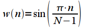 |
High resolution window |
| Lanczos window, or sinc - window |
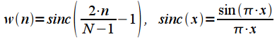 |
High resolution window |
| Bartlett window, or triangular window |
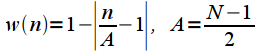 |
High resolution window |
| Hanna window |
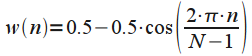 |
High resolution window |
| Barlett - Hanna window (Bartlett – Hann window) |
 |
High resolution window |
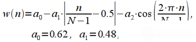
| Hamming window |
 |
High resolution window. The best window when  |
| Blackman window |
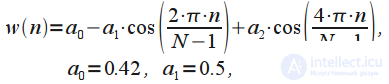 |
High resolution window. |
| Blackman – Harris window |
 |
Low resolution window |
| Natalla window (Nuttall window) |
 |
Low resolution window |
| Blackman – Nuttall window |
 |
Low resolution window |
| Flat Top Window |
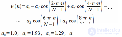 |
Low resolution window |
| Gaussian window (Gaussian window) |
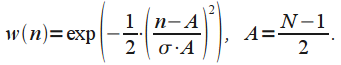 |
Window properties are parameter dependent.  |
Properties of window functions listed in Table 1 are shown in Table 2.
Table 2. Properties of some window functions
| Window Name |
 |
 |
 |
 db db |
 db db |
| Rectangular window (rectangle window) |
2 |
0.89 |
one |
-13 |
0 |
| Sine window |
3 |
1.23 |
1.5 |
-23 |
-3.93 |
| Lanczos window, or sinc - window |
3.24 |
1,3 |
1.62 |
-26,4 |
-4.6 |
| Bartlett window, or triangular window |
four |
1.33 |
2 |
-26,5 |
-6 |
| Hanna window |
four |
1.5 |
2 |
-31,5 |
-6 |
| Barlett - Hanna window (Bartlett – Hann window) |
four |
1.45 |
2 |
-35,9 |
-6 |
| Hamming window |
four |
1.33 |
2 |
-42 |
-5.37 |
| Blackman window |
6 |
1.7 |
3 |
-58 |
-7.54 |
| Blackman – Harris window |
eight |
1.97 |
four |
-92 |
-8.91 |
| Natalla window (Nuttall window) |
eight |
1.98 |
four |
-93 |
-9 |
| Blackman – Nuttall window |
eight |
1.94 |
four |
-98 |
-8,8 |
| Flat Top Window |
ten |
3.86 |
five |
-69 |
0 |
Gaussian window (Gaussian window)  |
eight |
1.82 |
four |
-65 |
-8,52 |
Gaussian window (Gaussian window)  |
3.4 |
1.2 |
1.7 |
-31,5 |
-4,48 |
Gaussian window (Gaussian window)  |
2.2 |
0.94 |
1.1 |
-15,5 |
-0.96 |
You can see the view of the above window functions and their frequency characteristics here.
findings
Thus, the issue of calculating the signal spectrum when observing on a limited time interval was considered. It is shown that the limitation of the analysis time is equivalent to the use of a rectangular window function, the frequency characteristic of which has maximum side lobes. A mechanism for reducing the level of side lobes by smoothing with a window is presented, which in turn worsens the resolution of the spectral analysis due to the expansion of the main lobe. The basic properties of the frequency response of window functions are shown, and expressions are given for the most common windows.

Comments
To leave a comment
Digital signal processing
Terms: Digital signal processing