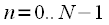
Lecture
 discrete signal samples
 . You need to resample and get
  discrete signal samples
  as shown in Figure 1. The sampling interval
  . Black shows the original signal, red - the result of resampling.
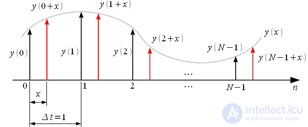 interpolate, i.e. continuous signal recovery
  then calculate its discrete values for each new
  . Interpolation can be done in various ways, in this article we will discuss polynomial interpolation. points passes a polynomial
  degrees
  and with only one. For example, through two points it is possible to draw only one straight line, through three points only one parabola, and so on. Respectively through you can also draw a single polynomial of degree which will be the result of interpolation, that is:
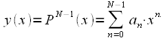 |
(one) |
 - coefficients of the polynomial, which must be calculated based on the signal samples
  Then substituting the necessary values resampling is possible.
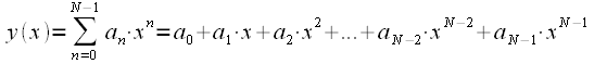 |
(2) |
for brackets: |
(3) |
for brackets: |
(four) |
for brackets, we get a set of nested brackets: |
(five) |
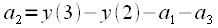
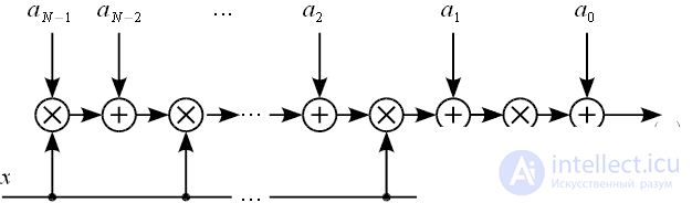 at known coefficients
 then added
  the “innermost brackets” of the expression (5) is obtained
 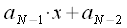 . "Innermost brackets" are multiplied by and so on all the brackets are collected and it turns out
  .
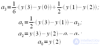
. . Get the cubic polynomial:
 |
(6) |
 based on discrete readings
  . To do this, you can create a system of linear equations:
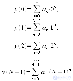 |
(7) |
. In addition, to solve the system of equations, matrix inversion is required, which is impossible to provide in real time, since for matrix inversion  multiplication operations. Thus, to construct a cubic polynomial with 64 multiplications required! Of course, such an approach cannot be applied in practice. Next, the Farrow filter for constructing a cubic polynomial using only three multiplications will be considered. can be represented as the sum of the product of its counts to the corresponding Lagrange polynomial
  :
: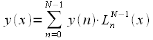 |
(eight) |
equal to one with  where
where  - sampling time
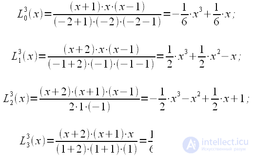
  - of the first counting and equal to zero at other moments of discretization. Figure 4 shows the cubic Lagrange polynomials for
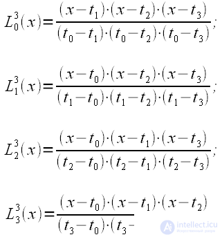
  . Each of the polynomials is equal to one at one of the sampling times and is zero in the others (this is indicated by markers). signal samples used different polynomials. Each Lagrange polynomial can be written in the form:
|
|
(9) |
and  sampling points. and sampling points
 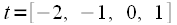 :
: |
(ten) |
 |
(eleven) |
 |
(12) |
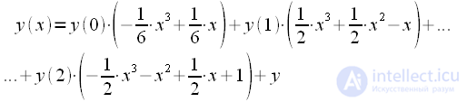
. using cubic Lagrange polynomials (12). With expression (8): |
(13) |
 in expression (13) is the sum of cubic polynomials, which means also cubic polynomial with coefficients ,
  .
. |
(14) |
, we get a cubic polynomial: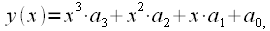 |
(15) |
 |
(sixteen) |
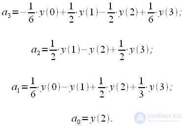
 depend on the four previous values. Thus, the coefficients of polynomial (15), in accordance with formula (16), can be obtained using FIR filters of the third order. Figure 5 shows an example of calculating a polynomial coefficient.
  using FIR filter.
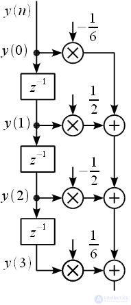 using a third order FIR filter
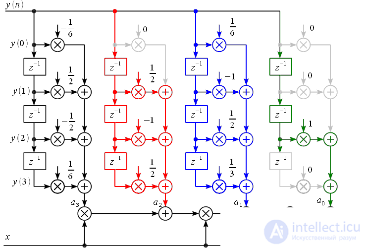 - black
  - red
- red  - blue
  - green. Gray marked branches multiplied by zero, which can be discarded from the scheme. According to the scheme, it is easy to calculate that the calculation of all coefficients of a polynomial requires 9 non-trivial multiplications (multiplication by zero and
  considered trivial). This is not 64 as required for the direct solution of the system of equations, but not three as stated above.
 |
(17) |
 |
(18) |
 |
(nineteen) |
 |
(20) |
 |
(21) |
 |
(22) |
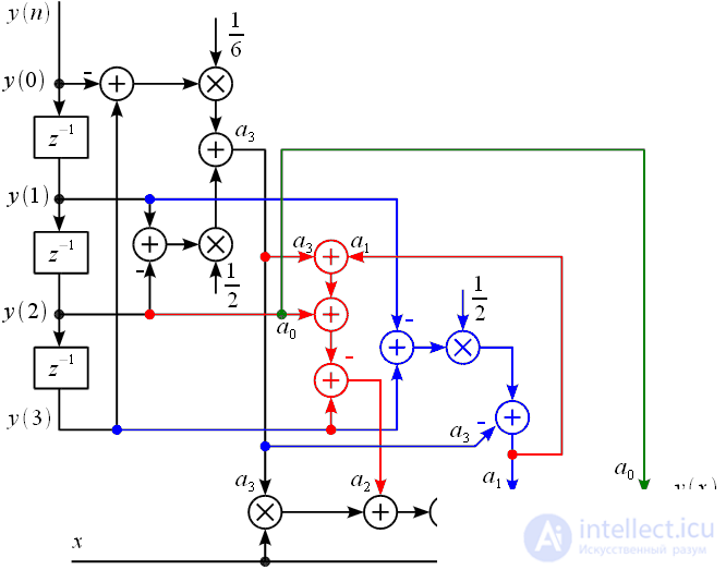 (black branches), then it is used to calculate the coefficient
  blue branches. Further coefficients and used to calculate
  . Coefficient
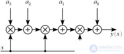
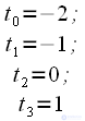
  just removed after the second delay. required to be calculated . The filter was synthesized based on the following initial data: there are 4 samples taken at time points . Accordingly, in order to get the value of the polynomial value
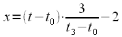
  should be in the range of -2 to 1, while
  corresponds to the sampling time
  , but
, but  corresponds to the sampling time
  . Value must be recalculated in the interval from -2 to 1.
 ,
,  ,
,  ,
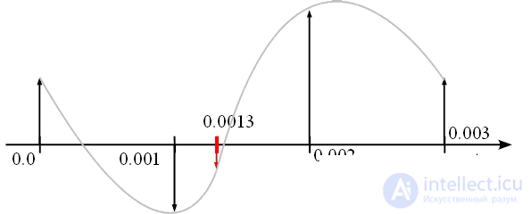
,  taken at a sampling frequency of 1 kHz, i.e.
  sec,
sec,  sec,
sec,  sec and
  sec (Figure 8). Calculate the value of the signal at time
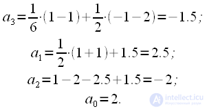
  sec
sec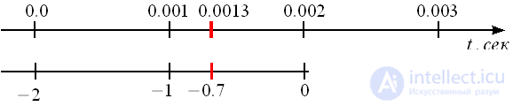
 |
(23) |
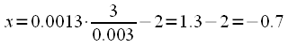 |
(24) |
 |
(25) |
equally: |
(26) |
 Or
Or  . In the previous example, it is impossible to calculate the signal value from these four samples, for example, for
  , because . Of course, it is possible to calculate more precisely, but the value will not correspond to reality. With the greatest accuracy, the signal values are calculated at normalized from -1 to 0. In practice, you should strive to recalculate the time scale in the interval from -1 to 0.
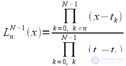

Comments