
Lecture
The Helmholtz machine (named after Hermann von Helmholtz and his concept of Helmholtz free energy) is a type of artificial neural network that can account for the hidden structure of a dataset by learning to generate a generative model of the original dataset. It is hoped that by learning an economical representation of the data, the underlying structure of the generative model should reasonably approximate the hidden structure of the dataset. The Helmholtz machine contains two networks, a bottom-up recognition network that takes data as input and produces a distribution over the hidden variables, and a top-down "generative" network that generates values of the hidden variables and of the data itself.
Helmholtz machines are usually trained using an unsupervised learning algorithm, such as the wake-sleep algorithm. They are the predecessors of variational autoencoders, which are instead trained using backpropagation. Helmholtz machines can also be used in applications that require a supervised learning algorithm (for example, character recognition or position-invariant recognition of an object in a field).
These networks are very different in architecture and in how they are trained.
The Helmholtz machine contains two networks: a bottom-up recognition network that takes data as input and produces a distribution over the hidden variables, and a top-down "generative" network that generates values of the hidden variables and of the data itself.
Boltzmann machines are much simpler, and their units are simply divided into "visible" units, V, and "hidden" units, H. The visible units are those that receive information from the "environment," i.e. our training set is a set of binary vectors over the set V.
Helmholtz machines were created to increase robustness to the noise that is always present in natural data, and in the hope that, by learning an economical representation of the data, the underlying structure of the generative model should reasonably approximate the hidden structure of the dataset.
The two phases of the Boltzmann machine contrast the statistics of the network's activations when input patterns are presented with the statistics of the network's activations when it is running "free." This contrastive procedure involves significant noise and is therefore slow to perform.
Helmholtz machines are trained using the so-called "wake-sleep" algorithm ( http://www.gatsby.ucl.ac.uk/~dayan/papers/d2000a.pdf ), in which the wake and sleep phases are not contrasted. Rather, the recognition and generative models are forced to chase each other.
The Helmholtz machine also has an interesting connection to the Boltzmann machine, which can be viewed as an undirected belief network.
In the Boltzmann machine, a potentially extended Gibbs sampling process is used for recognizing and generating input data, since nothing is as simple as the single-pass, directed recognition and generative belief networks of the Helmholtz machine.
Furthermore, the Boltzmann machine learning rule performs true stochastic gradient ascent on the log likelihood using a contrastive procedure that, confusingly, involves wake and sleep phases that are very different from the wake and sleep phases of the wake-sleep algorithm.
To summarize, these models are related in that both use representational learning, but for many problems Helmholtz machines simply provide convenient approximations.
A growing body of behavioral and neurophysiological evidence suggests that the brain performs optimal (or near-optimal) probabilistic inference and learning during perception and other tasks. Although there are many machine learning algorithms that perform inference and learning in an optimal manner, a complete description of how one of these algorithms (or a new algorithm) could be implemented in the brain is currently lacking. Many solutions have been proposed for how neurons might perform optimal inference, but the question of how synaptic plasticity might implement optimal learning is rarely addressed. This paper aims to bridge the two fields of probabilistic inference and synaptic plasticity by using a neural network of realistic spiking neuron models to implement a well-studied computational model called the Helmholtz machine. The Helmholtz machine lends itself to a neural implementation because the algorithm it uses to learn its parameters, called the wake-sleep algorithm, uses a local delta learning rule. Our spiking neural network implements both the delta rule and a small example of a Helmholtz machine. This neural network can learn an internal model of continuous training datasets in an unsupervised manner. The network can also perform inference over the learned internal models. We show how various biophysical features of the neural implementation constrain the parameters of the wake-sleep algorithm, such as the duration of the wake and sleep learning phases and the minimum sampling duration. We investigate deviations from optimal performance and relate them to properties of the synaptic plasticity rule.
Humans and other animals live in a predictable and structured environment, where they must make fast and efficient decisions in order to obtain food, escape predators, and find a mate. However, these sensory inputs provide only a limited and often distorted snapshot of the environment surrounding the animal. Although decisions are made using this imperfect information, they must reflect the true nature of the environment, since it is the environment that determines the effect of the animal's actions.
Bayesian inference provides a mathematical description of how to make optimal decisions given this limited and distorted information about the environment (Bishop, 2006; Griffiths et al., 2010). There is a large body of experimental evidence showing that humans and other animals behave in accordance with Bayesian inference in probabilistic tasks such as cue combination (van Beers et al., 1999; Atkins et al., 2001; Ernst and Banks, 2002; Alais and Burr, 2004; Burge et al., 2010), combining uncertain evidence with prior knowledge (Tassinari et al., 2006), sensorimotor learning (Körding and Wolpert, 2004), motion illusions (Weiss et al., 2002), and causal relationships (Blaisdell et al., 2006). Optimal learning has also been observed over development (Griffiths and Tenenbaum, 2006) and experimentally (Orbán et al., 2008; Chalk et al., 2010). Analysis of neural recordings during perception of natural scenes over the course of development is also broadly consistent with optimal inference (Berkes et al., 2011). This evidence motivates the search for an implementation of Bayesian inference in the brain.
In this framework, the brain maintains a probabilistic model of the physical laws that translate the composition of the environment (e.g., the objects in front of the animal) into the (distorted) sensory information that arrives at the brain (Figure 1A, bottom). As originally proposed by Helmholtz (1925), the brain then inverts this probabilistic model, also called a generative model, to produce a recognition model that transforms this distorted information into an optimal estimate of the composition of the environment, about which the brain can then make decisions (Figure 1A, Top). Learning in this framework involves tuning the parameters of the generative model (and hence its inverse, the recognition model) so that they match the statistics of the environment. Because exact Bayesian inference is generally intractable (Bishop, 2006), an approximate recognition model is often required. This approximation will manifest in the animal's behavior as certain behavioral biases (Sanborn et al., 2010).
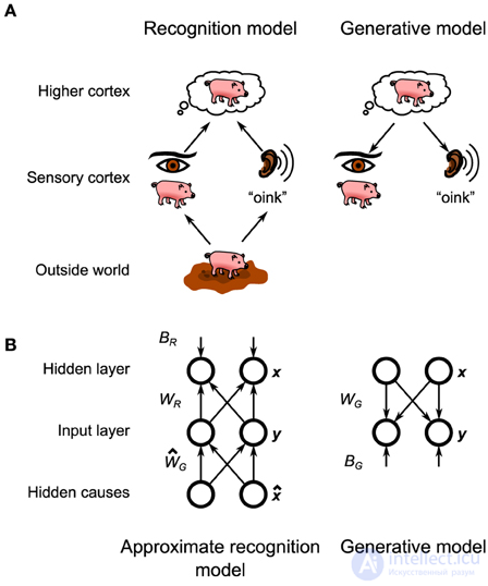
Figure 1. General view of the Helmholtz machine. (A) The hypothesized Helmholtz machine in the brain consists of two separate models: a recognition model and a generative model. The recognition model transforms neural activity in the early sensory cortices (produced by objects in the external world) to tune neural activity in higher cortical layers, which represent the hypothesized structure of the external world. The generative model runs in the opposite direction, transforming neural activity in higher cortical layers (produced by top-down connections from even higher cortical areas) into neural activity in the sensory cortex, which represents the reconstructed sensory stimulus corresponding to the world imagined by the higher cortex. (B) The Helmholtz machine in this paper consists of two input nodes and two hidden nodes. The model learns the recognition weights, W_R, and biases, b_R, as well as the generative weights, W_G, and biases, b_G.
We are interested in studying Bayesian inference at the level of neural implementation. This provides two benefits. First, the neural substrate adds an additional level of approximation and bias that can help in interpreting behavioral data, as noted above. Second, the neural specification of the algorithm will determine the type of data that should be looked for in neural recordings. There have been several proposals for how to implement Bayesian inference in neural networks (Lee, 2002; Friston and Kiebel, 2009; Moran et al., 2013), and some of these have advanced toward the use of spiking neurons (Rao, 2005; Ma et al., 2006, 2008; Shi and Griffiths, 2009; Buesing et al., 2011; Pecevski et al., 2011). Most of these past attempts did not address the question of learning. More recently, proposals have been developed for implementing both inference and learning in model neurons with stochastic (Brea et al., 2011; Rezende et al., 2011; Nessler et al., 2013) and deterministic (Deneve, 2008a,b) spiking mechanisms. We propose an alternative formulation (described in detail below) based on neurons with deterministic dynamics, with the required stochasticity arising from stochastic release at synaptic vesicles.
In this paper we address both the inference and learning questions by providing a spiking neuron model implementation of a specific algorithmic model of Bayesian inference called the Helmholtz machine. The Helmholtz machine (Dayan et al., 1995; Hinton et al., 1995; Hinton and Dayan, 1996; Neal and Dayan, 1997; Dayan, 1999, 2000) provides a method for performing both approximate inference and learning in a way that lends itself to biological implementation, because, unlike equally powerful models, changes in connection strength depend only on local correlations. In addition to the recognition model common to all implementations of Bayesian inference, the Helmholtz machine postulates the existence of an explicit generative model in the brain (Figure 1A). This generative model is not used during inference, but is crucial for learning the parameters of the recognition model (the recognition model, in turn, is used to train the parameters of the internal generative model). The original Helmholtz machine was successfully tested as a model of handwritten digit recognition (Hinton et al., 1995) and factor analysis (Neal and Dayan, 1997). The details of the biological implementation of these ideas have so far been incomplete, and the question of how to implement its learning rule, the delta rule, has been particularly troublesome. The proposed model will show how a microcircuit, combined with an experimentally observed rule of synaptic plasticity, can implement the computations needed to bridge the gap between the algorithm and the neural substrate.
The generative model that we will implement and use to model the (simulated) observed data is a mixture model of truncated Gaussians:

where x is the activity of the units in the hidden layer, and y is the activity of the units in the observed layer. The truncated Gaussian form is given by the following probability distribution function:

for some mean μ, covariance matrix Σ, and normalizing factor Z.  ( z ) is the multivariate Heaviside function:

where H(·) is the standard Heaviside function (with H(0) = 1), and the product is taken over all components of z.
The goal of perception, formulated within the Bayesian framework, is to invert this generative model, i.e., to find P( x | y ). In general this is intractable, so an approximate recognition model is used. In this case, the approximate recognition model is also a mixture of truncated Gaussians:

Both models have a fixed bias unit activity β and variance matrix Σ. The remaining parameters, namely the generative weights W G, biases B G, recognition weights W R, and biases B R are learned by the model using the wake-sleep algorithm. The values of the fixed parameters, as well as the initial values of the learned parameters, are detailed in Table S1. Since the variance parameters are not learned, the exact functional form of the mixture components is not essential (for example, a Poisson distribution would result in an identical neural implementation), as long as its mean depends linearly on the weights and biases. We chose the truncated Gaussian for mathematical convenience.
Exact wake and sleep learning rules for truncated Gaussian units can be derived by following a standard procedure (see Supplementary Information). During the wake phase of the algorithm, the generative model is adapted to the environment, first by estimating the activity of the hidden layer x (n) given the observation y (n) from the environment, using the approximate recognition model, and then adjusting the generative weights and biases as follows:
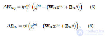
where η is the learning rate. During the sleep phase, the approximate recognition model is adapted to better invert the generative model, first by generating a sample { x (n) , y (n) } from the generative model, and then adjusting the recognition weights and biases:
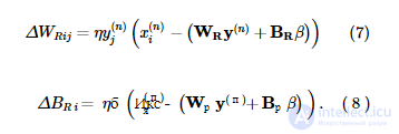
During training we constrain B R and B G to positive values, while W G and W R are left unconstrained.
Our neural network model will implement the above learning rules by approximating them using biologically plausible rules of synaptic plasticity (Figure 2). To focus our analysis on the difference between the computational implementation and the implementation using a neural substrate, we also use an approximate learning rule in the computational model (i.e., we do not use Equations 5–8). Given the target activity T, the input activity I, and the output activity O, let the error signal be M = max( T - O , −θ). The weight is then adjusted as follows:

where θ is some threshold activity. Equations (5, 6), for example, are approximated by the formula
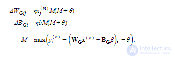
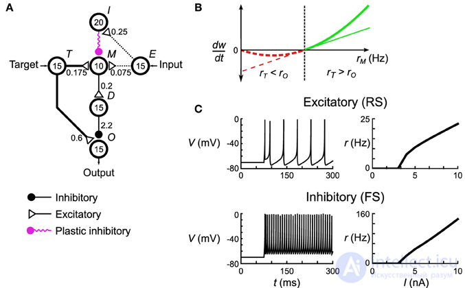
Figure 2. Implementation of the delta rule in a neural network. (A) The microcircuit implementing the delta rule consists of interconnected pools of neurons (circles). The numbers in the circles denote the number of neurons in each pool. The numbers next to the connections indicate the maximum total conductance along that pathway in nS. Connections have a sparsity of s = 0.3. Not shown are the nonspecific external connections made to each neuron in pools M and O. Each individual postsynaptic neuron in these pools receives its own Poisson spike train at a rate of r_ε = 100 Hz, which excites it via excitatory synapses with conductances of 0.42 nS and 0.6 nS, respectively. (B) The spiking plasticity rule at the plastic inhibitory synapses implements a form of the BCM rule. Synapses are depressed (dashed red lines) or potentiated (solid green lines) depending on whether the postsynaptic firing rate r_M is lower (or higher) than some threshold rate r_θ (bold line). By driving r_M to be below r_θ when the delta rule (thin line) predicts depression, and vice versa when the delta rule predicts potentiation, this microcircuit approximates the delta rule. (C) Responses of the model neurons to a constant current injection. When the neurons exceed a certain threshold current, their firing rate becomes approximately linear, which results in the overall linearity of this microcircuit.
This approximation can be obtained by assuming that unit activity is encoded using Poisson spike trains and that connection weights are adjusted using realistic rules of synaptic plasticity (see Supplementary Information). The quality of this approximation was verified empirically.
To model spiking neurons, we use the two-variable spiking neuron model proposed by Izhikevich (2003). The model is described by two coupled ordinary differential equations and one threshold condition:
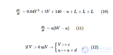
where V is the membrane potential (measured in mV), u is the adaptation current, and a, b, c, d are parameters determining the dynamics of neural excitation. We use two sets of parameters to model excitatory (regular spiking — RS) neurons and inhibitory (fast spiking — FS) neurons (Table S2).
I e models the excitatory current flowing through AMPA and NMDA receptors:

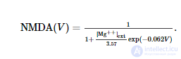
where g e1 and g e2 are the total dynamic conductances (measured in nS) of all excitatory synapses on the neuron. NMDA( V ) describes the dependence of the NMDA current on the membrane potential (Jahr and Stevens, 1990):
I i models the inhibitory current flowing through GABAA channels:
where g i is the total dynamic conductance (measured in nS) of all inhibitory synapses on the neuron.
I r is the current originating from excitatory synapses (modeled as AMPA currents) that are external to the network:
where g r is the dynamic conductance (measured in nS) of these external synapses.
Each time a non-external presynaptic neuron fires, after some delay Δ, the conductance of the corresponding synapse type is adjusted by a random amount:
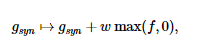
where w is the synaptic weight (measured in nS), and f is the number of vesicles released during the event. The distribution of f is modeled by a binomial distribution (Castillo and Katz, 1954) with a fixed number of vesicles, N v, and a release probability, P v (Table S2). For computational convenience, we approximate this binomial distribution by a normal distribution with mean N v P v and variance N v P v(1 - P v), truncated at 0.
External synapses are modeled as a Poisson process with rate r r Hz. When an external "neuron" fires, the conductance g r is adjusted by a fixed amount w r.
Between spikes, all of the above conductances evolve according to ordinary first-order differential equations:
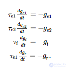
Delta-rule networks are subdivided into homogeneous pools of neurons denoted by labels (Table S3, Figure 2). Each network has an input pool E, an output pool O, and a target pool T, which are used to provide input to and read output from the network. In addition, there are intermediate pools M and D used by the network to perform computation and learning (see Results). Pairs of neuron pools are connected by directed sparse connections (Table S4). Each neuron in the source pool is connected to the same fraction of neurons in the target pool. The total conductance of the synapses created by a presynaptic neuron is fixed, and each synapse receives an equal share of this total. The connection sparsity, S, is the same for all connections between pools.
The spiking BCM synaptic plasticity rule estimates the postsynaptic spike rate. rˆr^post (measured in Hz) by filtering the sequence of postsynaptic spikes using an exponential kernel:
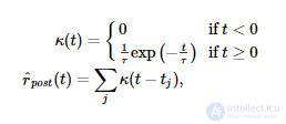
where t j is the time of the j-th postsynaptic spike. During each presynaptic event (which occurs at time t i for the i-th presynaptic spike) the synaptic weight is adjusted as follows:

The STDPi synaptic plasticity rule computes an estimate of the presynaptic spike rate, rˆr^rate pre- and of the postsynaptic spikesrˆr^post (both measured in Hz) by filtering the pre- and postsynaptic spike sequences, respectively, using a difference-of-exponentials kernel:
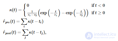
where t i is the time of the i-th presynaptic spike, and t j is the time of the j-th postsynaptic spike. During each presynaptic event the synaptic weight is adjusted as follows:

During each postsynaptic event the synaptic weight is adjusted as follows:
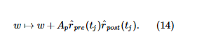
Plastic weights must remain non-negative.
To study the properties of the two plasticity rules, we construct two artificial spike trains. The presynaptic spike sequence is generated using a homogeneous Poisson process with constant rate r pre . The postsynaptic spike sequence is generated using an inhomogeneous Poisson process with postsynaptic spike rate r post ( t ):
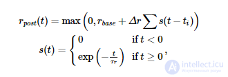
where t i is the time of the i-th presynaptic spike. In constructing this we use r post , which is the average over time of r post ( t ). We vary the base r to produce the required r post . These parameters are listed in Table S1.
To set the target rate and the input rate, we vary r r for the neurons within pools T and E, respectively. We keep the rate constant throughout the training and testing period. The output rate is computed by averaging the activation rate of all neurons within the output pool O during testing. During the testing period plasticity is turned off (for example, by setting the corresponding plasticity change amplitudes to 0).
The neural-network implementation of the Helmholtz machine consists of four units arranged in two layers. These units correspond exactly to the units x and y of the computational model . Each module has the same connectivity as the delta-rule network, except that pool E is removed, pool R is added, and variables labeled by the output pools X 1 , X 2 , Y 1 , Y 2 are added (Table S3). In addition, pool Iis now connected to the source pool rather than the target pool (although the connectivity is the same). These subunits are connected to one another by creating excitatory projections from the output pool and inhibitory projections from the pool I of a unit in one layer to the pool M of an element in the other layer (Table S4).
Inputs to the network arrive entirely through setting the r r variable of pool T to r T . During the wake phase r T is set equal to y ( n ) 1 and y ( n ) 2 for units y 1 and y 2 and equal to r ns for units x 1 and x 2 . During the sleep phase the reverse occurs: r T is set to x ( n )1 and x ( n ) 2 for units x 1 and x 2 and to r ns for units y 1 and y 2 . In addition, the connectivity between the units changes between phases, as detailed in Table S4.
Probability distributions over the output rates are computed by calculating a histogram of samples collected from the network. A sample is computed by averaging the rate of all neurons in the corresponding output pool over the sample duration, T sample .
The generative tests and the reward test use priors drawn from two families of unimodal and bimodal priors:


The parameters used for these prior distributions are listed in Table S5.
The decoding test uses a uniform prior:

where  ( z ; a , b ) is a sample of the uniform distribution of z over [ a , b ], and δ (·, ·) is the Kronecker delta. In constructing this we collect N test samples from each distribution.
The computational model and the neural network are trained on a set of 10 datasets, with the first eight used for the generative model tests and the last two for the decoding test and the reward test, respectively. The datasets are generated prior to training (and reused for all models) by drawing N test samples from the probability distributions. We chose the training distributions so as to avoid low firing rates, where our learning rules are least accurate.
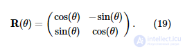
During training, data points are taken sequentially and in the same order for all trials (restarting from the beginning when the dataset is exhausted). The unimodal datasets a … e are drawn from a truncated Gaussian distribution:

The bimodal datasets f … i are drawn from a mixture of two truncated Gaussians:
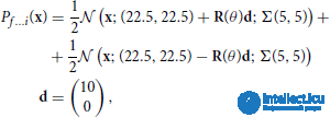
where Σ (ρ 1 , ρ 2 ) and R (θ) are defined in equations (18, 19). The parameters for these distributions are detailed in Table S6.
The dataset o for the decoding task is drawn from a uniform linear distribution with added truncated Gaussian noise:
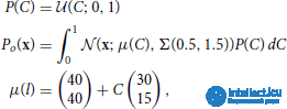
where ( z ; a , b ) is a sample of z from the uniform distribution over [ a , b ], and Σ (ρ 1 , ρ 2 ) is defined in equation (18). The data points are labeled with the value of the variable C, used to generate them.
The dataset r for the reward task is drawn from a uniform linear distribution:

where δ (·, ·) is the Kronecker delta. The data points are labeled with the value of the variable C, that was used to generate them.
We compute the similarity between two probability distributions P ( x ) and Q ( x ) using the Jensen-Shannon divergence ( Lin, 1991 ):
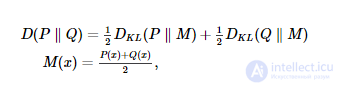
where D KL is the Kullback–Leibler divergence ( Kullback, Leibler, 1951 ):

We use base 2 for the logarithm, so that D lies in the range from 0 to 1. Since in most cases we do not have access to the full probability distribution, we estimate D by computing it between two two-dimensional histograms. The histograms have 40 bins on each side (1600 bins in total) and span the range from 0 Hz to 60 Hz. This method of computing D is biased ( Treves and Panzeri, 1995 ), but it is accurate enough for the purposes of this paper.
Given a sample x ( n ) from the computational model or from the neural network, we decode the presented valueCˆ( n )C^(n) by projecting this sample onto the line formed by the prior:
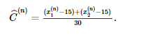
We can then compute the mean deviation as follows:
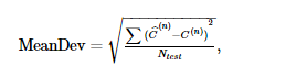
where C ( n ) is the label associated with y ( n ), which was drawn from the dataset and generated x ( n ) .
We decode the presented value  using a method similar to that of the decoding test (except for a different prior):
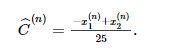
We then compute the response probability, 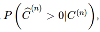 of the model, by applying a logistic function to it:

We interpret μ as the decision threshold, and s as a measure of the system's internal noise.
We compute the reward obtained by the model as follows:
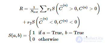
where r 1 and r 2 are the rewards associated with the two options. Because there is a symmetry in the Helmholtz machine, we swap x 1 and x 2, to flip the interpretation of all trials, if such a flip increases the computed reward.
If we assume that the system noise is distributed as a logistic distribution, then given the decision threshold μ and the internal scale of the system noise s, the reward achieved by the noisy decoder is:
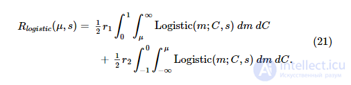
The optimal threshold μ opt is obtained by maximizing the logistic R :
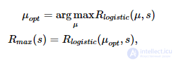
where the noise scale is estimated from the model for trials where r 1 = r 2 . The minimum reward that can be obtained given our scoring methodology is:
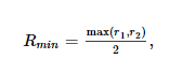
which can also be obtained by computing the corresponding limit of equation (21).
This task is particularly prone to convergence problems, so we discarded models whose decision thresholds fell outside the range [ Q 1 - 1.5 IQR , Q 3 + 1.5 IQR ], where Q 1 and Q 3 are the first and third quartiles, and IQR = Q 3. - Q 1.
The computational model was simulated using custom code written in the D programming language ( Alexandrescu, 2010 ) and run on the authors' personal computer. The neural network simulations were carried out using a neural simulator written by the authors in the D programming language. The simulator uses OpenCL ( Stone et al., 2010 ) to run on both GPGPU resources (an AMD Radeon HD 5830 on the authors' personal computer) and CPU resources (a high-performance computing cluster at Brandeis University). The source code for all models is available on the author's page.
Model fitting for the reward test was carried out using the SciPy package ( Jones et al., 2001 ) and the Python programming language ( van Rossum and Drake, 2001 ).
The specific Helmholtz machine implemented in this paper consists of two observable units y and two hidden units x (Figure 1B ). Here, "observable" means that the given unit directly receives sensory data from the environment (thus observing the environment), while "hidden" means that it does so indirectly (i.e., the environment is hidden from it). In practice, observable units may model early sensory areas of the brain, while hidden units may model later sensory areas. Each unit encodes a single continuous non-negative quantity. The generative model and the approximate recognition model are parameterized by generative weights, generative biases, recognition weights, and recognition biases.
The weights and biases are learned using an unsupervised learning algorithm called the wake-sleep algorithm ( Hinton et al., 1995 ). It consists of two quasi-symmetric phases: wake and sleep. During the wake phase, samples y ( n ) are taken from the training dataset and used to generate samples x ( n ) from the approximate recognition model. The generative weights and biases are then used to reconstruct the training data, and the reconstruction error is used to adjust the generative weights. Our model uses the delta rule for this purpose:
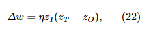
where z I is the value of the input unit (in this case, one of the hidden units), z O is the value of the output unit (in this case, the reconstructed training data for one of the observable units), and z T is the target value (in this case, the true value of the training data). w can be either the weight between two units at different layers (in this case, the top-down generative weight) or a bias weight, in which case the value of the input unit is taken to be β. During the sleep phase, samples x ( n ) are drawn from a prior distribution (equivalently, they are drawn from the distribution over the hidden units, conditioned on the activity of higher brain areas). They are then passed through the internal generative model to generate samples y ( n ) . The recognition weights and biases are then adjusted using the same rule (see Equations 5–8 in the Methods section).
Each unit of the computational Helmholtz machine is implemented using a circuit of spiking neurons (Figure 2A ). This network consists of small pools (10–20 neurons each) that form sparse but specific connections (see Table S4 for connectivity parameters) with one another. The network interacts with other units through an input pool (labeled E ), an output pool (labeled O ), and a target pool (labeled T). We interpret the average firing rate of the neurons in these pools (averaged over individual neurons) as the input, output, and target activity of the unit implemented by this neural network. The input and target pools are implemented as Poisson spike-train generators, while the remaining neurons in the network follow the dynamics described in equation (10). On a short timescale, the network implements the conditional distribution of the units (equations 1, 4); that is, the output rate r O is stochastically drawn from a distribution that is a function of the input rate r E and the internally encoded weights (encoding is discussed below). On a longer timescale, the network, through synaptic plasticity, adjusts the mean of r O(averaged over this longer timescale) to match r T in accordance with the delta rule (equation 22).
These two behaviors are implemented using the remaining pools in the network, labeled I , M and D . The overall architecture of the network is governed by the constraint that r O does not depend (as far as possible) on r T over a short time period (since the conditional distribution implemented by the network has no such short-term dependence), despite the fact that r T makes connections to the circuit implementing the delta rule (in our model neurons communicate exclusively via spikes). This is achieved by having the pool T form an excitatory connection with pools M andO , while having the pool M connect to the pool O through an intermediate inhibitory pool D . This arrangement is aided by the approximately linear FI curves of the component neuron types (Figure 2C ). The overall effect of this connectivity is that if the connection strength from pool E to pool M is excitatory, then an increase in r E will lead to a decrease in r O . The opposite occurs if the connection is inhibitory. Thus, this balance between excitation and inhibition with feed-forward connectivity implements the weight of the computational unit to which this network corresponds.
Pools I and M are responsible for adjusting this balance in accordance with the delta rule. The synaptic strength of the connections formed by the neurons of pool I with pool M is regulated by a spike-based plasticity rule that implements (under appropriate conditions) a particular rate-based form of the BCM rule ( Bienenstock et al., 1982 ). This rule regulates the synaptic strength based on the presynaptic firing rate ( r I ) and the postsynaptic firing rate ( r M ):
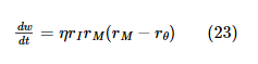
In the classical formulation of the BCM rule, r θ would depend on the average value of r M over a long period of time, but in our model it remains constant. The circuit implements the delta rule by applying the following two constraints. First, when r T ≥ r O , this means that r M ≥ r θ . Second, when r T < r O , this means that r M < r θ. Given these rate-ratio identities, the sign of the weight change that arises from the BCM synaptic plasticity rule (equation 23) for given r I , r O and r T , matches the sign arising from the delta rule (equation 22). In this way, the network approximates the linear form of the delta rule (Figure 2B , thin line) with the nonlinear form of the BCM rule (Figure 2B, bold line). Beyond preserving the sign, this is a fairly crude approximation, and verification will be needed to ensure that it still works correctly in tasks where it is meant to replace the delta rule. We want to emphasize that this approximation will be used well beyond the approximately linear region near r θ ; that is, we do not linearize the BCM rule around r θ . Apart from these plastic connections, the remaining synaptic connections are fixed, optimized to implement the constraints mentioned above.
To fully specify the spiking neural network in Figure 2A, it is necessary to clarify what is meant by rate (since it has no model-independent definition for spiking neurons), and the precise nature of the spike-based synaptic plasticity rule that implements the rate-based BCM rule required for the operation of the circuit described above.
In this paper we compare two spike-based rules that implement the BCM rule for particular classes of pre- and postsynaptic spike trains. The first is a minimal but biologically unrealistic implementation, which we call the Spiking BCM rule. The second is a simplified version of triplet-based, timing-dependent plasticity that is already known to be able to implement the BCM rule ( Pfister and Gerstner, 2006 ). We call this reduced version inhibitory, spike-timing-dependent plasticity, or STDPi .
The Spiking BCM rule estimates the postsynaptic rate  by filtering the sequence of postsynaptic spikes using an exponentially decaying kernel (Figure 3A , left). During each presynaptic spike, the synaptic weight is potentiated or depressed depending on the instantaneous value of
  (Figure 3C , left). The synaptic weight is not adjusted in any way during postsynaptic spikes.
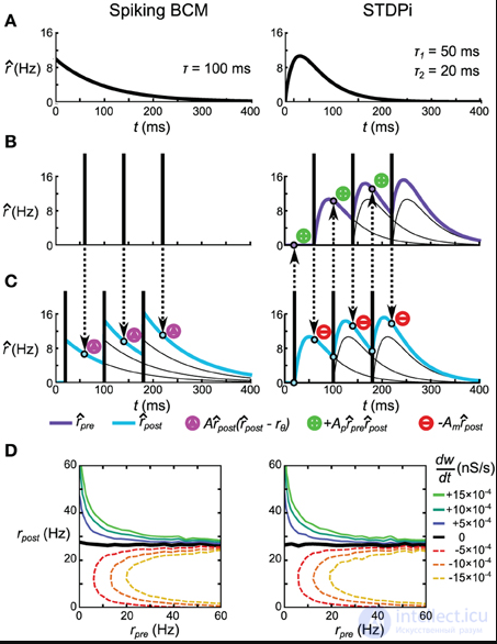
Figure 3. Spike-based plasticity rules that implement the rate-based BCM rule. (A) Kernels used to estimate the presynaptic (STDPi only) and postsynaptic (both rules) rate. The kernel for Spiking BCM is a single exponential rise and decay with one time constant, while the kernel for STDPi is the difference of two exponentials. Both kernels are zero for t <0. (B, C) Schematic diagram of the operation of the two rules for a given presynaptic spike sequence (B) and postsynaptic spike sequence (C). The magenta triangles shown indicate that Spiking BCM adjusts the synaptic weight (both in the positive and in the negative direction). The green plus signs and red minus signs shown indicate that STDPi respectively potentiates and depresses the synaptic weight. (D) dw/dt dw/dt as a function of uncorrelated, Poisson-distributed pre- and postsynaptic rates.
The STDPi rule filters both the presynaptic spike train and the postsynaptic spike train with a difference-of-exponentials kernel (Figure 3A , right) to estimate both the pre- and postsynaptic rate (rˆpre and  respectively). During presynaptic spikes the weight is decreased in proportion to the instantaneous value of
  . During postsynaptic spikes the weight is potentiated in proportion to the product of the instantaneous values of
  and rˆpre . This differs from the Spiking BCM rule, where potentiation and depression occur only during presynaptic spikes. In this sense STDPi more closely resembles experimental plasticity curves ( Haas et al., 2006 ). This rule is similar to the simplified triplet STDP rule studied by Pfister and Gerstner (2006), differing in the shape of the kernel (their work used an exponential kernel, as in the Spiking BCM rule) and in the fact that only a single trace is used to estimate the postsynaptic rate (as opposed to two in their work).
If we take two uncorrelated, Poisson-distributed pre- and postsynaptic spike trains and run them through these two rules, we see that they give identical values for  as a function of the rate of these spike trains (Figure 3D). This equivalence depends only on the values of A , A m and A p and τ, but not on the time constants of the STDP kernels. Furthermore, it can be seen that the presynaptic rate affects only the magnitude of
  but not its sign, unlike in the BCM rule (Equation 23). In fact, for Poisson-distributed spike trains both rules exactly implement Equation 23. See the Supplementary Information for the full derivation of these facts.
To implement the Helmholtz machine (Figure 1B), we organize four delta-rule networks, or units, as we will now call them (Figure 4; for clarity only three modules are shown), into two layers and establish connections between modules of different layers. Two of these units correspond to the variable y (sensory layer), while the other two correspond to the variable x (hidden layer). Since the delta-rule network operates on the firing rate of neuron pools, the neural network implementation of the Helmholtz machine encodes the values of these variables by rate coding. In this network, the mean rates (over a 500 ms window) of pools X 0 , X 1 , Y0 and Y 1 (collectively, the output pools) represent realizations of the random variables x 0 , x 1 , y 0 and y 1 respectively. The probability distribution over these variables is modeled through the stochastic variability of these rates, arising both from variations in the rate of the nonspecific external inputs to the M and O pools of the delta rule (see the legend to Figure 2 and Methods), and from stochastic release of synaptic vesicles at the network's synapses. By construction, the output pools are sampled (see Figure S1) from a probability distribution conditioned on the rate of the input pools (i.e., the output pools of the other units), weighted by the synaptic strength of the connections they make onto the M pool of each unit. In addition, there are pools that form plastic connections onto input pools that are nonspecifically active. These connections model the biases in the computational model. See Table S4 for details of the connectivity parameters. The computed weights and biases (namely W G , W R , B G and B R) correspond to the overall effect of the output signals of the modules on the firing rate of the units to which they connect. In terms of the neural network implementation, this corresponds to the balance between feedforward inhibition and excitation.
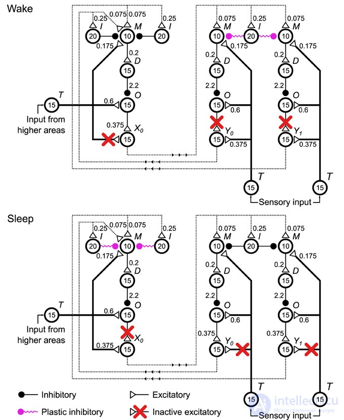
Figure 4. Configurations of the spiking neural network implementation of the Helmholtz machine during the wake and sleep phases of training. Four delta-rule networks (Figure 2A), referred to in the context of this network as units, are connected together to form the Helmholtz machine, two of which handle the sensory-level computations and two the hidden-layer computations (only one is shown in this figure for clarity). See the legend to Figure 2 for an explanation of the symbols used. To support the two phases of the wake-sleep algorithm, some connections (red crosses) are deactivated to control what determines the firing rate of the output pools of each unit (pools X 0 , X 1 , Y0 in this figure). In the wake phase (top), the outputs of the sensory units are determined by the sensory input, while the outputs of the hidden units are determined by the firing rate and corresponding connection strength of the outputs of the sensory units. In the sleep phase, the outputs of the sensory units are determined by the firing rate and corresponding connection strength of the outputs of the hidden units, while the outputs of the hidden units are driven by input from higher-order areas. Furthermore, in accordance with the wake-sleep algorithm, the strength of the plastic connections to the sensory units changes only during the wake phase, and conversely, the strength of the connections to the hidden units changes only during the sleep phase. Nonspecific external inputs within each unit are not shown. Also not shown are the plastic inputs to pool M of each unit, which implement the bias and weights. These are modeled as a Poisson spike train with rate r b = 25 Hz. These plastic inputs form the same plastic inhibitory synapse as all the other plastic connections shown in the figure.
Specific external connections are made through pool T of each unit (collectively, the external input pools). These are modeled as Poisson-statistics spike trains. In this case, the rate of these processes remains constant for each 500 ms interval, after which a new rate is drawn from the probability distribution under consideration (the external world or prior values).
The neural network uses an adapted wake-sleep algorithm (Figure 5, Training). To support the two stages of the training algorithm in this network, we introduced two sets of switchable connections. The first set includes the connections in each module that go from pool T to
продолжение следует...
Часть 1 The Helmholtz Machine and the Generative Model
Часть 2 4. Discussion - The Helmholtz Machine and the Generative Model

Comments