Quality assessment in classification tasks — is the process of measuring the effectiveness of a machine learning model in predicting the classes of objects. There are several standard metrics that are commonly used to evaluate classification quality:

1. Accuracy:

   • Shows the proportion of correct predictions relative to the total number of examples.
   • Formula: Number of correct predictions / Total number of examples

2. Precision:

   • Measures the proportion of correct positive predictions relative to all positive predictions. Formula: True Positives/(True Positives + False Positives )

3. Recall (Sensitivity):

   • Measures the proportion of correct positive predictions relative to all actual positive examples. Formula: True Positives/(True Positives + False Negatives )

4. F1-Score:

   • The harmonic mean of precision and recall. This metric is typically used when there is a need to account for both precision and recall. Formula: 2×(Precision×Recall)/(Precision + Recall )

5. ROC-AUC (Receiver Operating Characteristic - Area Under the Curve):

   • Measures the area under the ROC curve, which shows the relationship between the true positive rate and the false positive rate as the classification threshold changes.

6. Confusion Matrix:

   • A table comparing actual and predicted classes. It includes True Positives (TP), True Negatives (TN), False Positives (FP), and False Negatives (FN).

7. Specificity:

   • Measures the proportion of correct negative predictions relative to all actual negative examples. Formula: (True Negatives)/(True Negatives + False Positives )

8. Cohen's Kappa:

   • Measures the degree of agreement between the model's predictions and the actual values, taking chance agreement into account.

The choice of metrics depends on the specific task and business requirements. It is important to consider the context and the cost of errors depending on the goals of classification.

General Concepts

• TP — true positive: the classifier correctly assigned the object to the class in question.
• TN — true negative: the classifier correctly states that the object does not belong to the class in question.
• FP — false positive: the classifier incorrectly assigned the object to the class in question.
• FN — false negative: the classifier incorrectly states that the object does not belong to the class in question.

Here, when we talk about TP, TN, FP, FN and the concepts expressed through them, we are speaking within the context of a single class of binary classification. That is, in such a system it is implied that the actual number of objects of class 0 (for the binary case 0/1) can be expressed as TP₀ + FN₀ = FP₁ + TN₁

Confusion matrix (error / mismatch / loss matrix, CM)

Calculating TP, FP, FN from the CM

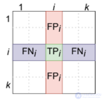
— is a square matrix of size k × k, where CMt,c — is the number of objects of class t , that were classified as class c , and k — is the number of classes. The values of the CM cells can be computed using the formula: 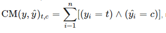, where yi — is the actual class of the object, and yi^ — is the predicted one.

For the binary case:

For multiclass classification, the confusion matrix is constructed following the same principle:

In this case, TP, TN, FP, and FN are calculated relative to some class (i) as follows:

Simple Quality Metrics in Classification Tasks

• Accuracy — (accuracy) shows the proportion of correct classifications. Despite its obviousness and simplicity, it is one of the least informative classifier metrics.

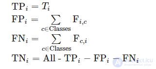
Acc=(TP + TN)/(TP + TN + FP + FN)

• Recall — (recall, sensitivity, TPR (true positive rate)) shows the ratio of correctly classified objects of a class to the total number of elements of that class.

Recall=TP/(TP + FN)

• Precision — (precision, the translation coincides with accuracy) shows the proportion of correctly classified objects among all objects that the classifier assigned to this class.

Precision=TP/(TP + FP )

• Specificity — shows the ratio of correct classifier responses to the total number of objects outside the class. In other words, how often the classifier correctly does not assign objects to the class.

Specificity=TN /(FP + TN)

• Fall-out — (FPR (false positive rate)) shows the proportion of incorrect classifier responses to the total number of objects outside the class. In other words, how often the classifier makes a mistake when assigning a given object to the class.

FPR=FP.(FP + TN)

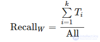
Given that such metrics do not take into account the original distribution of classes in the sample (which can significantly affect the resulting value), there are also weighted variants of these metrics (in terms of multiclass classification):

• Precision

• Recall

Different Types of Aggregation of Precision and Recall

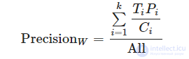
Examples and images are taken from the lectures of the course «Introduction to Machine Learning» by K.V. Vorontsov

Arithmetic mean:

Level lines for the arithmetic mean

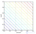
A=(1/2) *(precision + recall)

• If precision = 0.05, recall = 1, then A = 0.525
• If precision = 0.525, recall = 0.525, then A = 0.525.
• The first classifier — is constant, meaningless.
• The second classifier shows fairly good quality.

Thus, taking the arithmetic mean is not representative.

Minimum:

Level lines for the minimum

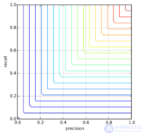
M = min(precision, recall)

• If precision = 0.05, recall = 1, then M = 0.05
• If precision = 0.525, recall = 0.525, then M = 0.525.

That is, it reflects the quality of the classifier fairly well, without overstating it.

• If precision = 0.2, recall = 1, then M = 0.2.
• If precision = 0.2, recall = 0.3, then M = 0.2.

But it does not distinguish classifiers with different non-minimal metrics.

Harmonic mean, or F-measure:

Level lines for the F-measure

• If precision = 0.05, recall = 1, then F = 0.1.
• If precision = 0.525, recall = 0.525, then F = 0.525.
• If precision = 0.2, recall = 1, then F = 0.33.
• If precision = 0.2, recall = 0.3, then F = 0.24.

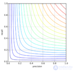
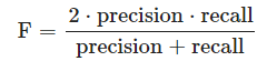
It is the most accurate averaging, taking both metrics into account.

Geometric mean, or the Fowlkes–Mallows Index (Fowlkes–Mallows index)

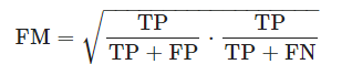
A less strict measure.

F-measure

For an overall assessment of classifier quality, the F₁-measure is often used. It is originally computed for the positive class in the binary classification case, and is generalized using the «‎one-vs-all» principle (described in more detail below, for multiclass classification). The F₁-measure — is the harmonic mean between precision and recall:

The weighted harmonic mean F_β (F₁-measure — a special case of the F_β-measure for β = 1). F_β measures the effectiveness of a classifier by weighting recall β times more important than precision:

F-measure for Multiclass Classification. Three Types of Averaging

The principle of averaging different F-measures for multiple classes

Calculating TP, FP, FN for multiclass classification

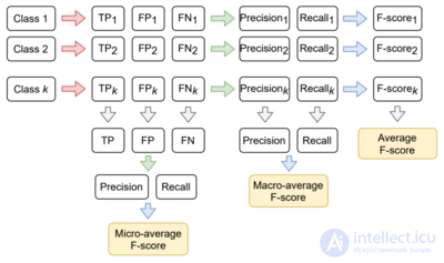
To calculate the F-measure (and other) metrics within multiclass classification, the «one-vs-all» approach is used: each class becomes «positive» exactly once, while the rest are — negative (an example of the calculation is shown on the matrix).

Thus, depending on the stage of computation at which averaging is performed, one can calculate the micro-average, macro-average, and average F-measure (the calculation logic is shown in the diagram on the right). Micro and macro:

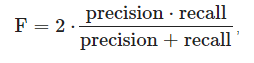
where for micro-average, precision and recall are computed from the averaged TP, FP, FN;

for macro-average, precision and recall are computed from the averaged precision_i, recall_i;

Averaged:

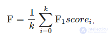
where i — is the class index, and k — is the number of classes.

ROC Curve

ROC curve; orange shows the ideal algorithm, purple — a typical one, and blue — the worst

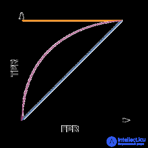
For a clear assessment of algorithm quality, the ROC curve is used. The curve is plotted on a plane defined by TPR (on the y-axis) and FPR (on the x-axis).

To plot the graph, soft classification is used: instead of definitively assigning an object to a class, the classifier returns the probabilities of the object belonging to various classes. This confidence is compared against a threshold (how much confidence is «enough» to assign an object to the positive class). Depending on the value of this threshold, the TPR and FPR values change.

Algorithm for constructing the curve:

1. Run the classifier on the test set
2. Sort the results by the classifier's confidence that the object belongs to the class
3. While there are elements left:
   1. Take the object with maximum confidence
   2. Compare the label with the actual one
   3. Recalculate TPR and FPR on the objects taken so far
   4. Plot a point if both metrics are not NaN / ±∞
4. Plot the curve through the points

Thus: the number of points does not exceed the number of objects; the ideal algorithm corresponds to an ROC curve passing through the point (0;1)(0;1); the worst algorithm (for example, a coin flip) corresponds to the straight line TPR = FPR.

To numerically evaluate an algorithm using the ROC curve, the value of the area under it is used (AUC, area under curve). The ideal algorithm has an AUC equal to 1, the worst — 0.5.

On the other hand, to construct an ROC curve it is not necessary to recalculate TPR and FPR.

There is an alternative algorithm for constructing an ROC curve.

1. sort the objects by the classifier's confidence in their belonging to the positive class
2. start at the point (0, 0)
3. sequentially continue the curve:
   • for each «negative» object, go up
   • for each «positive» one — go right.

The correctness of the algorithm is justified by the fact that, as the prediction for a single object changes depending on its class, either TPR or FPR changes (the value of the other parameter remains unchanged). Below, a different line of reasoning is described that leads to the algorithm above.

Accuracy graph for ideal classification

ROC curve for ideal classification

Accuracy graph for non-ideal classification

ROC curve for non-ideal classification

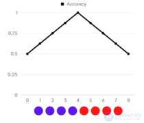
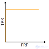
Recall that we are working with soft classification.

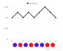
Let's consider examples (accuracy graphs, with color indicating the actual class of the object: red — positive, blue — negative). Let's sort our objects in increasing order of the classifier's confidence that the object belongs to the positive class. Suppose that the objects are located at an equal (unit) distance from one another.

Let's start moving the «decision boundary»: if the boundary is at zero — we decide to assign all objects to the positive class, so accuracy = 1/2. We successively shift the boundary one unit to the right:

• if the actual class of the object that has now ended up on the other side of the boundary — is negative, then accuracy increases, since we «guessed» the object's class correctly by deciding to assign objects to the left of the boundary to the negative class;
• if, on the other hand, the actual class of the object — is positive, accuracy decreases (by the same logic)

Thus, it can be seen on the graphs on the left that:

• on the graph of ideal classification, 100% accuracy is achieved, while for non-ideal classification — it is not;
• the area under the accuracy graph of the ideal classifier is greater than the corresponding area for the non-ideal one.

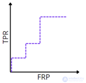
Note that by rotating the graph 45 degrees, we obtain the ROC curves for the corresponding classifiers (the accuracy graphs on the left correspond to the ROC curves on the right). This explains the alternative algorithm for constructing the ROC curve.

Precision-Recall Curve

PR curve

Rationale: Sensitivity to Class Ratio.

Let us consider the task of identifying mathematical articles from a set of scientific articles. Suppose there are 1.000.100 articles in total, of which only 100 relate to mathematics. If we manage to build an algorithm a(x)�(�), that solves the task perfectly, then its TPR will be equal to one, and its FPR — to zero. Now consider a «bad» algorithm that gives a positive answer for 95 mathematical and 50.000 non-mathematical articles. Such an algorithm is completely useless, yet it has TPR = 0.95 and FPR = 0.05, which is extremely close to the metrics of the ideal algorithm. Thus, if the positive class is significantly smaller in size, AUC-ROC can give an inadequate assessment of the algorithm's quality, since it measures the proportion of incorrectly accepted objects relative to the total number of negatives. For example, the algorithm b(x) placing 100 relevant documents at positions 50.001 through 50.101, will have an AUC-ROC of 0.95.

Precision-recall (PR) curve.

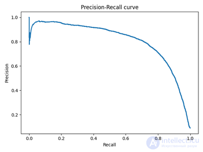
This problem of imbalanced classes can be avoided by moving from the ROC curve to the PR curve. It is defined analogously to the ROC curve, except that instead of FPR and TPR, the axes plot recall (on the x-axis) and precision (on the y-axis). The quality criterion for a family of algorithms is the area under the PR curve (English Area Under the Curve — AUC-PR)