
Lecture
Это окончание невероятной информации про машина гельмгольца.
...
the output pool. The second set includes the connections in each module that go from pool O to the output pool. These connections control what determines the realizations of the random variables: the rates r X 0 , r X 1 , r Y 0 , r Y 1 in this network. In the computational model, the realization y 0 , for example, can be drawn either from the environment or from the internal generative model. In the sensory units in the neural network, for example, this is determined by whether the active connection to the output pool is made from the external input pool, or from pool O . In the same spirit, these connections can be viewed as determining whether the unit generates a sample from its conditional probability distribution. For example, during the wake phase, to adjust the generative weights we compute W G x ( n ) + B G b(Equation 6), but we do not use this reconstructed mean value to generate a sample from the internal generative model. In the neural network, for example, during the wake phase the connection between pool O of the sensory unit and the output pool is broken, in order to prevent this sample from being sent to the hidden units. See the Discussion section for thoughts on the nature of these switching processes in the brain.
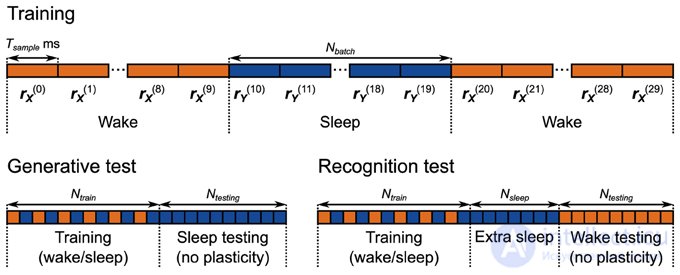
Figure 5. Training and testing protocols for the neural network implementation of the Helmholtz machine. The network is trained for 5000 s using alternating wake and sleep phases. Each wake and sleep phase consists of 10 samples of 500 ms each. During the generative test, 2000 samples are collected from the generative model.
Furthermore, the strengths of the connections to the sensory units (corresponding to the generative weights W G and biases B G ) change only during the wake phase, while the strengths of the connections to the hidden units (corresponding to the recognition weights W R and biases B R ) change only during the sleep phase. The sensory input and the input from higher-order areas during the sleep and wake phases respectively are set to a steady 40 Hz.
Unlike in the computational model, each wake and sleep phase here consists of several consecutive samples per phase. This is done to minimize the influence of the transient rate dynamics that occur when the network switches between the sleep and wake phases. For example, when the network switches from the wake phase to the sleep phase, the rate of pool M in the hidden modules (Figure 4) switches from operating on samples drawn from the environment to operating on samples generated by the generative model. Even though plasticity is switched off in these units during the wake phase, the kernels that estimate the firing rate of the neurons in these pools (Figure 3) continue to function. This means that initially, during the first sample of the sleep phase following a wake phase, the estimated rate is incorrect, which introduces errors into learning. A similar problem affects neighboring samples within the wake phase and neighboring samples within the sleep phase, but since the rates are drawn from the same distributions in each case (from the environment and from the prior, respectively), this is a less serious problem. These issues place limits on the timescale of the neuronal dynamics, the plasticity rules, and the mechanisms of active sensing (e.g., saccades). If the environment changes faster during the wake phase (or higher brain areas fluctuate in activity during the sleep phase) than the rate-estimation mechanism can keep up with, learning will be adversely affected.
This problem means that the choice of the number of samples per phase can be critical for successful learning. In practice, we find that this choice depends on the complexity of the data and the prior distributions. Difficult tasks (bimodal datasets and difficult priors) require larger batch sizes. We use a batch size of 10 for most tasks, increasing it to 50 for more demanding recognition tests. Our tests show that once the batch size exceeds a certain amount, network performance plateaus for a small (≤ 50) number of samples per phase.
To test the functionality of the delta rule neural network, we took 121 separate but structurally identical networks for each plasticity rule. Each network was given a different target rate r T and a different initial mean weight of the plastic connections w start . All other parameters remained the same, with r E , set to 20 Hz. We then simulated each network under these conditions and recorded r O . Before training, r O increased with increasing w start (Figure 6A , left). The change in r O as a function of r Tbefore training reflects the imperfect linearity of the network. After 50 seconds of training, r O now tracks r T, both when the network used the spiking BCM rule and when it used STDPi (Figure 6A , middle, right). Note that if we change r T on a short timescale, r O will remain unchanged (modulo the caveats mentioned above): the pattern of change in r O arises from the fact that r I affects it differently depending on the trained weights. To more clearly examine how well r O tracks the trained r Twe simulate 50 instances of random connectivity for each of the 121 networks described above, and average over the initial weights. For the spiking BCM rule, we note that the deviation between r T and r O is approximately constant for all r T (Figure 6B , red line), whereas for STDPi this deviation increases with increasing r T (Figure 6B , blue dashed line). If we look at the change in weight at w start = 1 (Figure 6C), we can see that this is because STDPi does not increase the synaptic weight as much as spiking BCM does under these conditions. This is not a convergence problem, since looking at the overall change in weight over time for a single trial, averaged over 50 networks, it becomes clear that the weights converge for both rules during training (Figure 6D ). Despite these shortcomings, at least in this simple task, using the approximate delta rule and implementing it with spiking plasticity rules does not lead to a catastrophic degradation in performance, and we can move on to attempting to use this network as part of the Helmholtz machine.
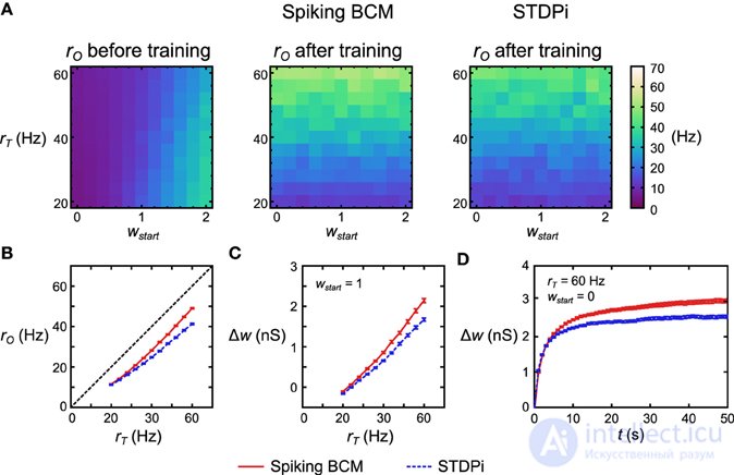
Figure 6. Performance of the delta rule neural network. (A) For each plasticity rule, 121 structurally identical networks were given different r T and initial weights w start . The networks were then simulated for 50 s. Before training, r O tracks w start and depends strongly on r T . After training, r O tracks r T (more precisely, it tracks the w that was trained by r T, since r O is largely independent of r Ton short timescales). (B) Averaging over 50 instances of the 121 delta-rule networks described above and collapsing along the w start axis, the deviation from r T is nearly constant for all values of r T when spiking BCM is used (solid red), but this is not the case when STDPi is used (blue dashed line). (C) Networks using the STDPi protocol fail to reach high weight values. (D) Change in weight over time for a single trial across 50 networks. For both plasticity rules, the weights approach a certain steady state, but for STDPi this final weight value is lower than for spiking BCM. Error bars are SEM.
We first test the computational model and the neural network in the generative regime. That is, we check how well the model matches the probability distribution over the input units on which it was trained. This is most applicable to matching spontaneous neural activity in vivo in early cortical areas (e.g., early sensory cortex, Berkes et al., 2011). The computational model and the neural network are trained on nine datasets (labeled a through i ). Datasets a through e consist of unimodal two-dimensional truncated Gaussians, with and without skew, while datasets f through iare bimodal mixtures of undistorted two-dimensional Gaussians. For the unimodal datasets we use a unimodal prior distribution (Equation 15), whereas for the bimodal datasets we use a bimodal prior distribution (Equation 16). In the neural networks, the different priors are implemented by changing the firing-rate distribution of pool T in the hidden units during the sleep phase. This manual, task-dependent choice of priors is necessary because our model contains only a single hidden layer; the strength of the Helmholtz machine lies in its ability to be implemented in a hierarchical structure, so that the type of prior can be learned as the connection strength for a second hidden layer in a larger model.
The models are trained and tested according to the protocol shown in Figure 5., Generative test. Each session begins with a training period of total duration 5000 s (a total of 500 wake phases and 500 sleep phases, where each phase comprises 10 samples) for the neural network. The computational model is trained for 250,000 wake and sleep phases (one sample per phase). We use a relatively higher learning rate for the neural network for the sake of computational efficiency. At the same time, however, it is 90% slower than it was in the delta rule network, because the weights do not converge properly if the learning rate is too high. This was not a problem in the delta rule network, owing to the constant input it received during training. The order of data presentation was randomized for each session (see Materials and Methods). At the end of each session, after training, we probe the generative model of both the neural network and the computational model by collecting 2000 samples from it. We examine 50 separate networks, each with a different instance of random connectivity, in order to study the effect of the connectivity issues described above. We record one such session for each network.
We first investigate how the neural networks perform when trained on unimodal datasets (Figure 7A , first column) with a unimodal prior (Figure 7B ). For comparison, we also examine histograms of the generative models obtained from the computational model trained on the same datasets and with the same priors (Figure 7A , second column). Despite using an approximate learning rule (Equation 9) the computational model manages to accurately learn the generative models. We quantify this by computing the similarity between the generative models and all the training datasets. We measure similarity using the Jensen-Shannon divergence (Lin, 1991)., which ranges from 0 for absolutely identical probability distributions to 1 for non-overlapping distributions. We look at D net, which is the average divergence across the datasets, and D pop, which is the average of D net across all the random instances of the model.
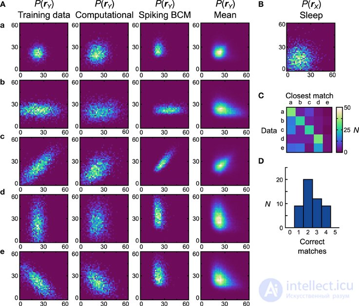
Figure 7. Performance of the neural network implementation of the Helmholtz machine with the spiking BCM rule on unimodal datasets. (A) The computational model and 50 instances of the neural network were trained on the five unimodal datasets shown in the first column. Axes range from 0 to 60 Hz on both components of r Y . The resulting generative models from the computational model are shown in the second column. The generative models of the best-performing (in terms of the match between the training-data distributions and the learned generative models) neural network are shown in the third column. The fourth column shows the population-averaged generative models of the neural networks. (B) The prior distribution used for the generative models. Axes range from 0 to 60 Hz on both components of r X . (C) Confusion matrix obtained by matching the generative models of individual networks against the mean (computed across all networks for a given dataset) generative distributions. (D) Histogram of the number of correct matches for each neural network.
After computing the similarity matrix, we look at the dataset that is most similar to the generative model, and if it matches the dataset that was used for training, we say that the model correctly learned the dataset. By this metric, the computational model correctly learned all the datasets presented ( D net = D pop = 0.19). For the neural network implementation, we examine the two plasticity rules separately. We generate 50 separate networks, each with a different instance of random connectivity, and examine the performance across these network implementations. Starting with the networks that used the spiking BCM rule, the generative models of the best network (i.e., the one that produced the highest number of matches) are shown in Figure 7A., third column ( D net = 0.35). Across all instances, the neural implementation failed to match dataset e ( D pop = 0.39 ± 0.012 SEM).
Dataset e poses a problem for the neural network because it requires the components of yto be anticorrelated, which in this model can only be achieved with negative generative weights. The delta rule network is able to represent negative weights by adjusting the balance between excitatory and inhibitory feedforward input connections. However, the range of weights it can represent is not symmetric about zero, making it impossible to obtain the very negative weights needed to model certain distributions. The reason for this asymmetry lies in the fact that only the inhibitory connections are plastic in our network. A strongly negative weight requires strong feedforward excitation, which is difficult to counteract with plastic inhibition when non-negative weights are required. Therefore, relatively weak feedforward excitation is used, which results in a limited capacity to represent negative weights. This problem could be solved by using a more sophisticated population coding scheme (see Discussion). We therefore do not expect this to be a relevant problem for the brain.
Since the networks produced generative models quite different from the datasets on which they were trained, it is more informative to compute the similarity matrix relative to the probability distributions obtained by averaging the generative models of all the networks trained on a given dataset (Figure 7A). , fourth column). This analysis will show whether the generative models learned by the networks differ across datasets. If the networks perform this task perfectly, then the mean-distribution dataset to which a network's generative model is most similar will match the dataset on which that network was trained. We can depict this using a confusion matrix (Figure 7C). for all the neural networks. We see that for the first four datasets, most networks produce generative models that match the mean distribution well, but fail when trying to match the mean distribution of dataset e . A performance histogram showing the number of correct matches for each network (Figure 7D ) shows that no network matches all five datasets, and most networks match only two.
Next, we examine how the neuronal Helmholtz machines with the STDPi plasticity rule perform on the same unimodal datasets. When this rule was used in the isolated delta-rule networks, deviations in performance from the spiking BCM rule could already be observed, so we also expected different performance on this task. One of the findings from studying the delta rule network was that when it used the STDPi rule, it could not match high target rates (Figure 6B). . To compensate for this, we multiplied by three all the prior rates used both in the computational model and in the network with the BCM plasticity rule (the training datasets remained unchanged). An unfortunate side effect of this is that the detailed behavior of the network obtained with this rule can only be qualitatively compared with that produced by the spiking BCM rule.
Figure 8A shows the datasets (first column), the generative models of the best network (second column), and the mean distributions (third column). The previously used prior is shown in Figure 8B. The D net of the best network is 0.47 and D pop= 0.53 ± 0.13 SEM. It is clear that networks using STDPi have trouble matching the data even qualitatively (the best network correctly matches only the first three datasets). The networks tend to produce positively correlated probability distributions regardless of the training data, although the level of correlation is modulated in the correct direction. As before, we also examine how much the generative models trained on different datasets differ from each other by computing a confusion matrix (Fig. 8C) and the corresponding matching histogram (Fig. 8D). Despite the relatively low performance in matching the data distributions, the networks do learn distributions that differ when trained on different datasets. Five (10%) of the networks matched all five datasets, although, as with the Spiking BCM rule, most matched only two.
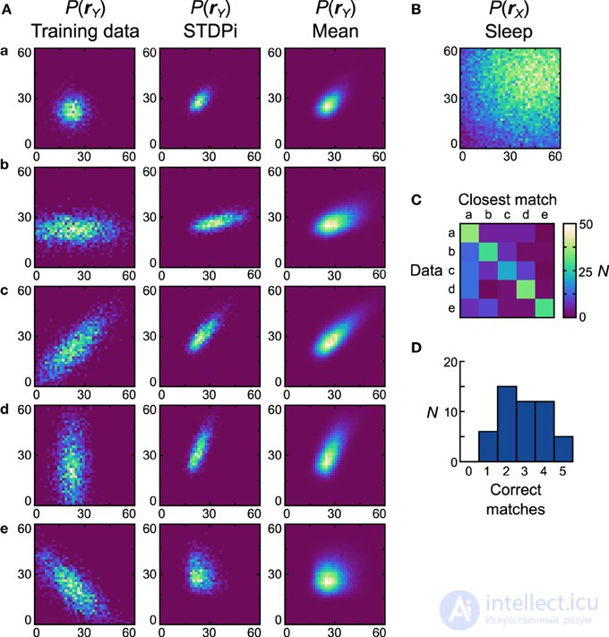
Figure 8. Performance of the Helmholtz machine neural network implementation with the STDPi rule and unimodal datasets. See Figure 7 for an explanation of the panels. Parameters for the STDPi kernels: τ1 = 50 ms, τ 2 = 20 ms.
Figures 7 and 8 were produced using bimodal datasets (Figure 9A, first column) and priors (Figure 9B). Again, the computational model has no trouble with these datasets (Fig. 9A, second column), resulting in close qualitative and quantitative matching (near-perfect matching performance using the matching test, D net = D pop = 0.30). Starting with the Spiking BCM plasticity rule, the generative models from the best-performing neural network (Fig. 9A, third column) qualitatively resemble the datasets on which they were trained, and although the matching performance is ideal, D netis relatively poor at 0.62 ( D pop = 0.58 ± 0.0075 SEM). Examining the mean distributions, it becomes clear that most networks perform poorly on dataset g. The reasons for this are similar to why neural networks perform poorly on dataset e, namely the need for strong negative connections. Running the matching test on the mean distributions yields a confusion matrix (Figure 9C) and a performance histogram (Figure 9D). Seven (14%) of the networks match all four mean distributions.
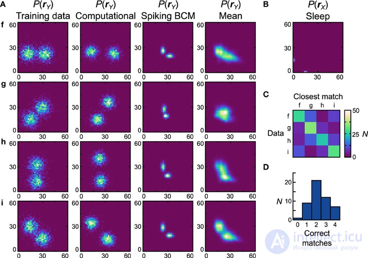
Figure 9. Performance of the Helmholtz machine neural network implementation with the Spiking BCM rule and bimodal datasets. See Figure 7 for an explanation of the panels.
Networks using the STDPi rule perform better on bimodal datasets (Fig. 10A, first column) and bimodal priors (Fig. 10B). The generative models of the best network appear qualitatively similar to the datasets (Fig. 10A, second column), although D net has a high value of 0.53 ( D pop = 0.59 ± 0.0082 SEM). The only exception is dataset g, which is difficult to learn because it relies on a good representation of negative weights. Looking at the confusion matrix (Fig. 10C) and the matching histogram (Fig. 10D) we see how much the learned distributions differ depending on which dataset they were trained on. Twenty-two (44%) of the networks correctly match all the mean distributions (Fig. 10A, third column).
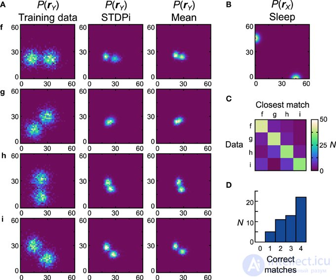
Figure 10. Performance of the Helmholtz machine neural network implementation with the STDPi rule and bimodal datasets. See Figure 7 for an explanation of the panels. Parameters for the STDPi kernels: τ1 = 50 ms, τ2 = 20 ms.
Overall, it appears that the transition from the computational model to the neural implementation affects performance in a nontrivial way. Despite the neural network implementation and the computational model using an approximate learning rule, the neural networks perform quantitatively worse on all the metrics shown here. This drop in performance is a combination of the shortcomings already shown in the results for the delta-rule networks (Fig. 6), together with the previously mentioned effects of crosstalk between learning stages and the imperfect switched connectivity. In addition, fundamental problems with weight representation affect some classes of data distributions but not others.
The STDPi and BCM plasticity rules are identical for certain classes of pre- and postsynaptic spike trains, and when used in the more complex and realistic setting of the delta-rule networks they also show relatively small quantitative differences. However, in the more complex setting of the neural Helmholtz machine, these small quantitative differences are amplified into qualitative effects. The STDPi rule performs relatively poorly when the networks using it must learn a probability distribution, and even providing a more favorable prior does not solve all the problems.
The explanation for the discrepancy between the apparent similarity of the Spiking BCM and STDPi rules shown in Figure 3C and their dissimilar performance in the delta-rule network and the Helmholtz machine lies in the short-term correlation between pre- and postsynaptic spike trains arising at inhibitory synapses (the corresponding excitatory synapses in this model are relatively weak). The kernels used to estimate the rates can be made less sensitive to these correlations by reducing the contribution of the parts of the kernel that are most affected by these correlations. Specifically, we adjust the shape of the kernel so that the interval immediately after a presynaptic spike contributes less to the rate estimate. We do this by changing τ 2, which determines the width of the initial dip of the STDPi kernel (Figure 3A). To show the overall effect this parameter has on the behavior of the rule, we examine two extreme values of τ 2 , 1 ms and 30 ms. The kernels for these values of τ 2 are shown in Figure 11A. For symmetry, we use the same kernel to estimate both the pre- and postsynaptic rates, although the postsynaptic kernel shape is largely irrelevant for this analysis. First, we verify that STDPi using both kernels produces the same behavior as shown by the original STDPi kernel (with τ 2 = 20 ms), as shown in Figure 3B, when the spike trains are uncorrelated. Figure 11B shows that as the pre- and postsynaptic rates are varied, we obtain the same behavior for the two kernel shapes. We then generate a series of spike trains with short-term negative correlations. Spikes are generated from the rate expressions using a Poisson process (homogeneous in the presynaptic case and inhomogeneous in the postsynaptic case, see Materials and Methods). When we apply STDPi using the two different kernels to such correlated spike trains, we find, as expected, that the correlations do change the net synaptic plasticity as a function of the mean pre- and postsynaptic rates. In particular, the biggest change is an increase in the postsynaptic rate at which the synaptic weight remains unchanged over time (Fig. 11C, black line - uncorrelated, purple dashed line - correlated). This occurs because the presynaptic rate is underestimated, leading to less potentiation of the synaptic weights. Importantly, we see the benefit of a larger τ 2 (Fig. 11C , right panel), which improves not only the net underestimation of the presynaptic rate - and, hence, the average shift in the postsynaptic rate at which the synapses no longer change strength - but also the dependence of the position of the nullcline on the presynaptic rate. The latter is important, since to reproduce the ideal delta rule, the steady-state postsynaptic rate must be the only factor affecting the direction of change of that synapse.
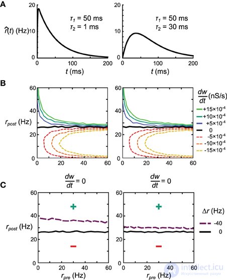
Fig. 11. Effect of kernel shape on the behavior of the STDPi plasticity rule. (A) The two kernel shapes considered in this figure. The same kernel is used for both the pre- and postsynaptic rate estimation. (B) dw/dt as a function of uncorrelated, Poisson-distributed pre- and postsynaptic rates for the kernel with τ 2 = 1 ms (left) and τ 2 = 30 ms (right). (C) dw/dt = 0 nullcline for uncorrelated, Poisson-distributed pre- and postsynaptic spike trains (black), and for negatively correlated, Poisson-distributed presynaptic and inhomogeneous-Poisson postsynaptic spike trains (purple). The kernels used have τ 2 = 1 ms (left) and τ 2 = 30 ms (right). All other contour lines are omitted for clarity.
As described earlier, the results obtained on these artificial examples do not necessarily predict performance in real networks. We therefore examine how both the delta-rule network and the neural implementation of the Helmholtz machine depend on the choice of τ 2 .
For the delta-rule network, we quantify performance by looking at the average deviation of the output rate after training from the target rate. We vary τ 2 and look at the average deviation across 50 networks (differentiated by instances of random connectivity). We see that the deviation decreases as τ 2 increases (Fig. 12A). When τ 2 = 30 ms, the average deviation across the different networks is 12.50 ± 0.26 (SEM) Hz, which is slightly smaller than the average deviation of 10.98 ± 0.25 (SEM) Hz obtained using the Spiking BCM rule.
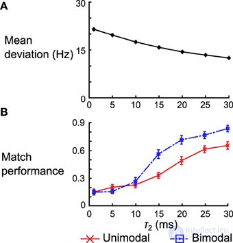
Figure 12. Effect of kernel shape on the performance of the delta-rule network and the neural implementation of the Helmholtz machine. (A) Average deviation (over 50 network instances) between the output rate after training and the target rate, across 50 instances of the delta-rule network. Error bars are SEM, but they are too small to be seen on this plot. (B) Average matching performance for unimodal and bimodal datasets across 50 instances of the neural implementations of the Helmholtz machine. Error bars are SEM. Note that performance is normalized by the number of datasets (for example, a performance of 1.0 means that all 5 mean distributions were matched in the unimodal dataset category).
For the neural implementation of the Helmholtz machine, we focus on the matching test performed in panel D of Figures 8 and 10. We look at both unimodal and bimodal datasets and normalize the network’s performance by the number of datasets in that group (that is, instead of ranging from 0 to 5 for unimodal datasets, it now ranges from 0 to 1). We examine the performance of 50 instances of the Helmholtz machine neural networks, varying τ 2, as before. While matching performance increases for both dataset types as τ 2increases, it increases far more sharply for bimodal datasets (going from matching an average of 1.26 datasets to 3.40 datasets). This is partly because networks using poor kernels typically fail to learn the weights that produce bimodal generative models. Once the kernels become good enough (τ 2 > 10 ms) to separate the two modes, performance increases sharply.
So far we have only tested our implementation of the Helmholtz machine in the generative mode. However, during behavior and perception, animals are most likely to use the recognition model to perform inference. We therefore now examine how well the neural networks perform in recognition mode. This mode is most applicable for comparison with neural data in higher cortical areas, as well as with behavioral data. In this section we focus on behavioral tasks, since behavioral data are more readily available.
The first test we perform is a simple linear decoding test. The models are trained using a uniform linear dataset (Figure 13A, dataset o ) and a prior (Figure 13B). During testing, the models must determine where the presented data point lies on the line (position in this case is a one-dimensional quantity ranging from -1 to 1). This is achieved by looking at where the activity of the hidden units lies on the prior (which is also a line). The critical point here is that the decoding strategy used to evaluate the model is explicitly specified by the prior distribution, meaning that the transformation from the data distribution to the distribution of decoded positions is learned entirely by the model (for details of the decoding procedure, see the Materials and Methods section). The models are trained and tested according to the protocol depicted in Figure 5, the recognition test. During each session, the computational model is trained for 50,000 phases (25,000 wake phases and 25,000 sleep phases), while the neural networks are trained for 5,000 s (500 wake phases and 500 sleep phases with 10 samples per phase). To test the performance of the computational model, it is simulated 50 times (with separate instances of temporal stochasticity). For the neural network, we generate 50 networks with different realizations of random connectivity for each plasticity rule. Each network is tested using a single session, as described above.
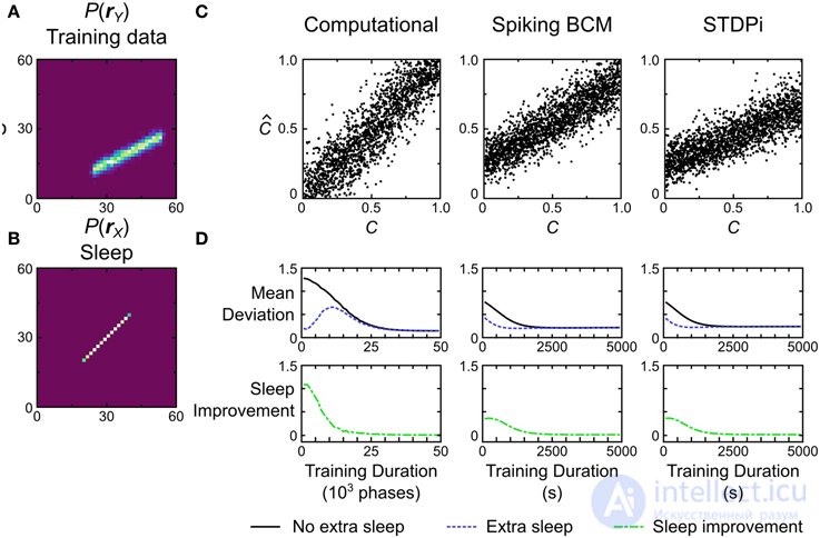
Fig. 13. Performance of the computational and neural network models on the decoding task. (A) The dataset on which the models are trained to perform this task. Each data point is labeled with a value C indicating its position on the line. The position ranges over [0, 1]. The models must recover this position from the data alone. (B) The prior distribution used during training. (C) Decoding performance of three example model instances. C is the true value used to generate the data point, and Ĉ is the value estimated by the model from the data. (D) If training is stopped before the weights converge, additional samples in the sleep phase without further presentation of data can lead to improved performance. Error bars are omitted for clarity.
Figure 13C shows the performance of the computational model and two instances of neural network models, one using the Spiking BCM plasticity rule and the other using the STDPi plasticity rule. The computational model performs decoding without any noticeable systematic bias, whereas the neural networks show a systematic bias and an inability to decode the full dynamic range of the data. We can quantify performance by computing the average deviation (defined as the square root of the mean squared error, averaged across trials) between the true positions of the data points and the decoded positions. The computational model shows the best performance at 0.15. Neural networks using the Spiking BCM rule perform worse, with an average deviation of 0.22. Networks with the STDPi rule perform slightly worse still, at 0.24.
This decoding test is a good way to illustrate a prediction arising from the means by which any implementation of the Helmholtz machine learns its recognition weights. Since performance on the task depends solely on the recognition weights, and the recognition weights are learned during the sleep phase, we can observe an improvement in performance during the sleep phase without presenting any additional training data. This is trivially true for the short sleep phases used during training, because without any improvement we would not observe an overall increase in performance across training as a whole, over both sleep and wake. However, this is not entirely the case for longer sleep phases with a larger number of samples. In the early stages of training, a long sleep phase will produce a convergent recognition model that inverts a not-yet-fully-converged generative model,
To study this effect, we first track the average deviation of the models during training (Fig. 13D, black curve). The initial weights for all models were chosen to be small, so the initial average deviation is correspondingly large. We use relatively lower learning rates for all models in order to visualize the improvement in performance over time, since this task is very simple and the models would otherwise learn it too quickly. At certain intervals we stop presenting data and repeat sampling in the sleep phase until the recognition weights converge. Examining the average deviation of the models (Fig. 13D, blue curve) shows a clear, sleep-induced decrease in the average deviation, without any new presentation of data. The green curve in Figure 13D shows the magnitude of this improvement at different times during training. Unsurprisingly, the greatest improvement occurs early in training, whereas late in training such extended sleep phases yield little benefit.
The second test we perform is a two-alternative forced-choice task with unequal rewards for the two options. We use a training dataset consisting of a set of uniform linear data (Figure 14A, dataset r) and a bimodal prior (for example, Figure 14B shows the distribution used for neural networks using the STDPi rule). We refer to the position along the data line as C (for consistency; see the Discussion and Figure 15 for the behavioral-task interpretation of this test), ranging from -1 to 1. During testing, the models must determine whether C is less than or greater than 0. This is achieved by noting which of the two hidden units has the greater activity (for example, whether y 1 ≥y 2 or y 1 < y 2 ). Thus, the models can only report whether C was greater than or less than 0. When the model correctly indicates that C > 0, it receives a reward with value r 1 , whereas if it correctly indicates that C <0, it receives a reward. with a different reward value r 2. The sum of the two reward values is constrained to 1, so an ideal noiseless decoder applied to noiseless data (as in this case) would receive an average reward of 0.5. The reward does not affect the plasticity rules - the Helmholtz machine uses an unsupervised learning algorithm - but it does affect the prior distribution (in the brain, the prior distribution in this case would be altered by reward-dependent plasticity). The two truncated Gaussians that are mixed to produce the prior distribution are mixed in the proportion r 1 / r 2 (Figure 14B shows the prior distribution with r 1 / r 2= 4). Thus, the activity of the hidden units represents the reward levels associated with the observed actions of the units. This task is difficult for the neural networks when the reward ratio is high (i.e., one mode is much larger than the other), so we train the networks for longer periods of time (7500 s) and use larger batches of samples (50) in each wake and sleep phase. As before, we simulate the computational model 50 times. For the neural network, we generate 50 networks with different instances of random connectivity, and then test each on the entire training dataset.
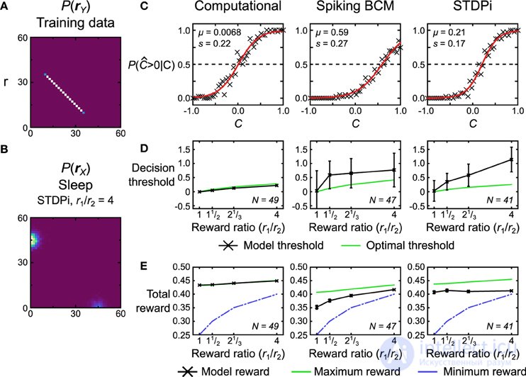
Figure 14. Model performance of the computational and neural network in the reward task. (A) The dataset r, on which the models are trained for this task. Each data point is labeled with C, denoting its position on the line. The position lies in the range [−1, 1]. Models must determine whether this position is positive or not, with the two alternative choices being rewarded with different amounts. (B) The bimodal prior for this task encodes the reward ratio r 1 / r 2 of the two alternative choices by modulating the weighting coefficients of two Gaussian blobs. The location and sizes of the Gaussian blobs are the same as in Figures 9 , 10.. The prior used for neural networks with the STDPi plasticity rule is shown, for r 1 / r 2 = 4. (C) Response probability of three example models for r 1 / r 2 = 1. The probability data (crosses) are fit with a logistic function (red line) to determine the model's internal noise and decision threshold. Note that the two neural networks show a shift in the decision threshold. (D) The model's decision threshold (black) compared to the optimal threshold (green), given the model's noise level (estimated from trials where r 1 / r 2= 1). Error bars represent standard deviation. N is the number of models used to build the plot. (E) Reward obtained by the model (black) compared with the maximum obtainable by an optimal decoder with a matched noise level (green), and the minimum possible given the scoring procedure (blue). An optimal noiseless decoder would obtain a reward of 0.5 under all conditions. Error bars are SEM. N is the number of models used for the plotted data points.
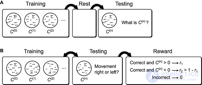
Figure 15. Possible behavioral tasks implementing recognition tests. (A) A possible behavioral task for testing the sleep-improvement prediction. First, subjects are shown moving dots with varying degrees of coherence. After training, subjects are allowed to rest. During subsequent testing, subjects are again shown moving dots with varying degrees of coherence, but now they are asked to report the coherence. If the brain uses a Helmholtz machine to learn recognition weights, then rest will lead to improved performance compared with the absence of a rest period between training and testing (Figure 13D ). (B) A possible behavioral task for studying the effect of reward bias on decision thresholds. Subjects are shown moving dots with varying degrees of coherence moving in one of two directions. At the same time they are asked which direction they perceive the moving dots to be going, and are rewarded differently depending on the true direction of motion. If the brain uses a Helmholtz machine to learn recognition weights for this task, then the subject's decision thresholds will be shifted relative to the optimal thresholds.
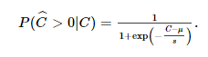
First, we quantitatively assess the performance of the models by examining how the response probability [ P (CˆC^> 0 | C )] depends on the true value of C . Figure 14C shows this data for a single run of the computational model and two neural network implementations, one using the Spiking BCM rule and the other using the STDPi rule. For these three plots the reward ratio is set equal to one. We fit the data with a logistic function, parameterized by its location μ, which we call the decision threshold, and its scale s, which measures the internal noise of the system:
The first observation is that both the neural and computational models are noisy and therefore cannot reach the theoretical maximal payoff of a noiseless decoder. This also means that the decision threshold will vary depending on the reward ratio: an optimal noisy decoder shifts the decision threshold away from the choice carrying the larger reward (see "Materials and Methods" for the derivation of this fact). Another observation is that the decision thresholds of the neural networks are not equal to zero even when the rewards for the two choices are equal (in which case the optimal threshold is 0). This is caused by random connectivity in the neural networks. We plot how this decision threshold changes as a function of the reward ratio (i.e.,14D ). Noise is estimated from trials with the reward ratio set to unity. The computational model adjusts its threshold nearly optimally, but the neural networks substantially overshoot the threshold, i. e., the more rewarding choice is selected even more often than is optimal. This phenomenon has been observed in experiments with monkeys ( Feng et al., 2009 ). We also look at the actual average total reward obtained by the models (Figure 14E , black curves). We can compare the obtained reward with the theoretical minimum and maximum reward (green and blue curves in Figure 14E., respectively). The maximum reward is achieved using the optimal threshold value and therefore depends on the model. The minimum reward is obtained if we choose the threshold so that the model always responds with the most rewarded choice. The computational model, in effect, obtains close to the maximum possible reward given its level of internal noise. The neural networks do not perform as well either. The low performance of the neural networks is partly due to the fact that the extremely simplified decoder we use to extract decisions from the neural networks does not take into account the bias arising from random connectivity. Thus, these results represent a lower bound on performance. This lower bound could be improved with some simple modifications to the decoder (adding homeostatic synaptic scaling (Turrigiano and Nelson, 2004 ), for example).
We presented a spiking neural network that implements the Helmholtz machine and its associated unsupervised learning algorithm, the wake-sleep algorithm. To build such a model, we also designed a smaller circuit that implements the delta rule, the error-correction rule that underlies learning in the wake-sleep algorithm. We showed that this model can learn a generative model that captures the probability distributions of the datasets on which the network was trained. In addition, we showed that it can perform approximate probabilistic inference in two recognition tasks. Throughout this work we contrasted two synaptic plasticity rules, Spiking BCM and STDPi, as candidate mechanisms for implementing the delta rule and obtaining the learning required in the Helmholtz machine. Although STDPi is based on biological observations,
The generative tests we performed can be used to explain data showing similarity between stimulus-evoked neural activity and spontaneous neural activity ( Han et al., 2008 ; Berkes et al., 2011 ; Okun et al., 2012 ), as well as providing a normative explanation for the replay of neural activity during sleep ( Sutherland and McNaughton, 2000 ). The two recognition tests can be applied to behavioral experiments in which subjects must observe a stimulus and then make decisions based on their inferred perception. Figure 15 shows two possible experiments using moving-dot displays that would reveal the results of the recognition tests. Figure 15A shows a decoding experiment that investigates the effect of rest (additional samples after training during a sleep phase) on decoding performance. Figure 15B shows a biased-reward experiment that investigates the suboptimal shifts in decision thresholds predicted by our model. Notably, experiments (with a slightly different task) showing suboptimal shifts in decision thresholds in monkeys already exist ( Feng et al., 2009 ).
The neural network we propose is not the first to implement the delta rule, although, as far as we know, it is the first to satisfy the requirements imposed by our neural network implementation (using rate-coded spiking neurons as a continuous variable and avoiding temporal causality) of the Helmholtz machine. By carefully controlling the postsynaptic activity of the synaptic connection, whose strength is otherwise regulated by a BCM-like rule, Hancock et al. (1991) applied a partial delta rule for binary units. This implementation is inadequate for this Helmholtz machine because it uses continuous-valued units. More recently, by combining spike-rate adaptation and spike-timing-dependent plasticity ( D'Souza et al., 2010) implemented the delta rule for temporally separated, but otherwise continuous, units. The nature of the temporal separation requires that the target activity appear after the network activity. Such temporal separation would require a violation of causality in any neural implementation of the Helmholtz machine, because in reality the target activity appears earlier than the activity produced by the network. For example, during the wake phase the target activity is set by the stimulus, while the current network activity arises from top-down connections that are driven by the stimulus. It is possible that delay lines or post-inhibitory rebound spikes could produce the necessary ordering of activity, but we chose an approach that did not require such additional complications.
As part of our choice of implementation for the Helmholtz machine, we also simultaneously chose to represent probability distributions using samples. This approach has previously been explored by others ( Fiser et al., 2010 ; Buesing et al., 2011 ; Pecevski et al., 2011 ; Nessler et al., 2013 ) and has a number of interesting theoretical properties (see Fiser et al., 2010 ; Lochmann and Deneve, 2011 for a review), and also lend themselves directly to the implementation of biologically plausible learning algorithms ( Nessler et al., 2013 and this work). A popular alternative represents probability distributions using probabilistic population codes ( Rao, 2005; Ma et al., 2006 , 2008 ). This framework has broad experimental support, although a biologically plausible learning algorithm for it has not yet been proposed. Another alternative for encoding probability distributions is spike-prediction coding ( Deneve, 2008a , b ), which supports both inference and learning at the level of individual neurons, but does not extend naturally to the representation of continuous variables.
The Helmholtz machine implemented in this paper is very simple and consists of only one input layer and one hidden layer, each with two linear units. As a result, many of the functions achieved by this particular instance and presented in this paper could be accomplished with simpler models without the need for elaborate circuitry and the wake-sleep algorithm. The strength of the Helmholtz machine, however, lies in its ability to scale up through the use of multiple layers and multiple units, as well as different conditional probability distributions ( Hinton and Dayan, 1996 ). We chose to limit ourselves to a very impoverished model in order to clarify how and why its performance is affected by the neural implementation. In addition, there exist more powerful extensions of the Helmholtz machine with within-layer connectivity (Hinton and Dayan, 1996 ; Dayan, 1999 ), which still use the wake-sleep algorithm. Further implementation of these ideas would allow the assumed connectivity of neural networks to more closely match the available neurophysiological data.
The connections between layers in our network are implemented using feedforward excitatory and inhibitory synapses, of which only the inhibitory ones are plastic. However, this is not a strict requirement. The same functions could be implemented even if both types of synapses are plastic, or only the excitatory synapses are plastic, for the reasons outlined below. A key constraint of the synaptic plasticity rules at the connection is that the net weight of the connection (resulting from the combination of the average inhibitory and excitatory conductance at the connection) is regulated as predicted by the rate-based BCM rule (Equation 23). In the delta-rule network, this means that when the postsynaptic rate is close to r θ (Figure 2B) and the net connection weight increases, the synaptic rules should produce a net decrease in this weight. This does not preclude excitatory synapses from being strengthened, but it does not mean that inhibitory synapses must be strengthened more . In this sense, we say that the plasticity of the network will be anti-Hebbian. We restricted ourselves to using only one type of plastic synapse in order to minimize the number of parameters. Evidence for anti-Hebbian rules is scarce for excitatory synapses (although see Sjöström and Häusser, 2006 and Letzkus et al., 2006 ), but exists for inhibitory synapses ( Haas et al., 2006).). In addition, prior theoretical work concerning probabilistic inference also suggests the use of anti-Hebbian plasticity at both excitatory and inhibitory synapses ( Rezende et al., 2011 ). However, unlike that work, our model predicts anti-Hebbian plasticity in both top-down and bottom-up connections.
Consistent with the ideas presented in this work, the kernels of the inhibitory synaptic plasticity rule found in the entorhinal cortex of rats by Haas et al. (2006) show a pronounced dip for nearly coincident pre- and postsynaptic spikes. The STDPi rule proposed in this paper goes beyond the experimental data, since it assumes a quadratic, BCM-like postsynaptic rate dependence (Figure 2B).), which was not investigated in the experiments. The experimental plasticity rule also has time constants that are shorter than required by well-performing STDPi kernels, but this may be explained by the biological neurons in the cell-dynamics experiments operating on a faster time scale than our model neurons. We predict that brain regions implementing the rate-based wake-sleep algorithm presented here will have adaptations (in the form of kernel shape or weight-change timing) to reduce the bias introduced by spike correlations.
Although our formalism is based on connections with pure anti-Hebbian plasticity, our model does not require that all connections in the brain be purely anti-Hebbian. Non-hierarchical generative models, such as models with lateral within-layer connections, may require alternative plasticity rules to learn these connection weights ( Dayan, 1999 ). On the other hand, not every part of the brain may require an explicit generative model and thus may be better described by other frameworks unrelated to the Helmholtz machine ( Brea et al., 2011 ; Nessler et al., 2013 ). Overall, our proposal is compatible with the abundance of known Hebbian plasticity rules in the cortex and hippocampus.
The wake-sleep algorithm is implemented in our model by reconfiguring the network for each phase. Such reconfiguration, however, need not be carried out in the brain through explicit synapse suppression or shunting. For example, the connection between pool O and output pool X 1, depicted in Figure 4, could be "switched off" by strongly inhibiting the cells in pool O without any reconfiguration of connectivity. This inhibition could be periodic, consistent with the abundance of rhythms in the cortex ( Buzsáki and Draguhn, 2004 ), although such clock-like periodicity is not required for the wake-sleep algorithm to function.
The wake and sleep phases may correspond to the animal's actual wakefulness and sleep. There is evidence of circadian fluctuations in modulators affecting learning ( Steriade, 2004 ; Welberg, 2013 ) and corresponding changes in observed neuronal firing patterns ( Sherman, 2001 ) and overall functional connectivity ( Massimini et al., 2005 ). Alternatively, rapid perceptual learning can occur without interruption of sleep ( Hawkey et al., 2004 ; Alain et al., 2007), suggesting that the wake and sleep phases may correspond to the state of the network when a relevant stimulus is present (and attended to), while the sleep phase represents the spontaneous state of the network (or a state of inattention). In this case, the required connectivity switches would be triggered by different network dynamics in states with different levels of attention. Such attention-dependent dynamics have been observed in a number of sensory areas of the cerebral cortex ( Fontanini and Katz, 2006 , 2008 ).
Our networks use sparse random connections between pools, but do not include homeostatic and structural plasticity mechanisms to adjust the non-plastic connections to counteract unfavorable realizations of random connectivity. In the worst case, a neuron may be completely disconnected from its upstream neurons or be tonically active. This contributes to large variability in performance across different network realizations and to overall suboptimal performance compared with the computational Helmholtz machine. We believe that, by contrast, near-optimal behavior in animals arises from the brain using such mechanisms ( Holtmaat and Svoboda, 2009 ; Vitureira et al., 2012), which, if added to our models, would likely help close the apparent gap in average performance between our networks and the experiments.
Our model uses a highly simplified coding strategy for representing continuous variables, whereby the average firing rate of a population of neurons is interpreted directly as the value of the variable. One consequence of this is that the variance of the encoded probability distribution of the variable is inversely proportional to the number of neurons used to encode it. By using relatively small pools of neurons, we introduce high variance. When this is detrimental to the task (e.g., Figure 13 ), we expect the brain to pool the actions of several single networks in order to reduce the variance in the decision outcomes.
Another issue arising from our coding strategy is the difficulty of representing negative weights, due to which the neural networks had trouble modeling probability distributions with negative correlations. Instead of a one-to-one correspondence between firing rate and stimulus variables, using a more sophisticated coding strategy (e.g., using ideas from Eliasmith and Anderson, 2003 ) within the framework of the Helmholtz machine is a natural extension of our work that could address such issues.
Throughout this paper we have represented samples from the probability distribution as the average rate of a pool of neurons over 500 ms. This is inconsistent with data showing that correlations between the activity of different neurons decay within 20-40 ms ( Berkes et al., 2011 ) and that perceptual decisions can be made on similarly short timescales ( Stanford et al., 2010).). The duration of each sample required for successful learning in our implementation depends critically on the timescale that the synaptic plasticity rules use to estimate the relevant rates. In our preliminary simulations we observed (data not shown) that the learning performance of the networks drops noticeably when samples are shortened in duration (the shortest sample duration we tested was 100 ms). The decrease was more pronounced for the STDPi rule than for the Spiking BCM rule, consistent with the overall lower performance of the former shown in this paper. However, these issues should only arise during training. Outside of training, shorter samples can be used, allowing the framework to model fast inference.
Overall, we think that the approach adopted in this paper for implementing the Helmholtz machine in a neural network is promising, and improvements to the model along the possible directions discussed above could provide a unified explanation of how probabilistic inference is performed in the brain.
Часть 1 The Helmholtz Machine and the Generative Model
Часть 2 4. Discussion - The Helmholtz Machine and the Generative Model

Comments