
Lecture
Autoencoder (also — autoassociator) — a special architecture of artificial neural networks that enables unsupervised learning using the backpropagation algorithm. The simplest autoencoder architecture — a feedforward network, without feedback connections, most similar to a perceptron and containing an input layer, a hidden layer, and an output layer. Unlike a perceptron, the output layer of an autoencoder must contain the same number of neurons as the input layer.
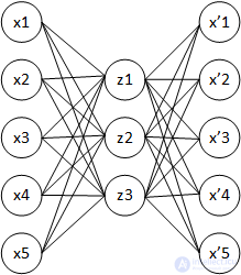
The basic principle of operation and training of the autoencoder network — to obtain, at the output layer, a response as close as possible to the input. To keep the solution from being trivial, constraints are imposed on the hidden layer of the autoencoder: the hidden layer must either be of lower dimensionality than the input and output layers, or the number of simultaneously active neurons in the hidden layer is artificially restricted — sparse activation. These constraints force the neural network to search for generalizations and correlations in the input data and to compress it. In this way, the network automatically learns to extract general features from the input data, which are encoded in the weight values of the artificial neural network. For example, when trained on a set of different input images, the network can learn on its own to recognize lines and stripes at various angles.
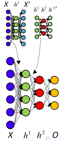
Autoencoders are most often applied in a cascade to train deep (multilayer) networks. Autoencoders are used for the unsupervised pretraining of a deep network. To do this, the layers are trained one after another, starting with the first ones. Each new, untrained layer has an additional output layer temporarily attached to it, completing the network into an autoencoder architecture, after which a training dataset is fed to the input of the network. The weights of the untrained layer and of the additional autoencoder layer are trained using the backpropagation algorithm. The autoencoder layer is then removed and a new one is created, corresponding to the next untrained layer of the network. The same dataset is again fed to the input of the network; the already-trained earlier layers of the network remain unchanged and act as the input for the autoencoder layer currently being trained. Training continues in this way for all layers of the network except the last ones. The last layers of the network are usually trained without an autoencoder, using the same backpropagation algorithm and on labeled data (supervised learning).
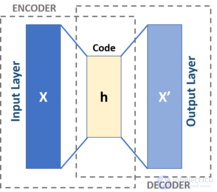
The simplest form of an autoencoder is a non-recurrent feedforward neural network, similar to the single-layer perceptrons that make up multilayer perceptrons (MLP), employing an input layer and an output layer connected by one or more hidden layers. The output layer has the same number of nodes (neurons) as the input layer. Its purpose is to reconstruct the input data (minimizing the difference between the input and the output) instead of predicting a target value given inputs
 . Therefore, autoencoders are unsupervised learning models. (They do not require labeled input data for training).
An autoencoder consists of two parts: an encoder and a decoder, which can be defined as transitions  and
and  such that:



In the simplest case, given a single hidden layer, the encoder stage of an autoencoder takes the input  and maps it to
  :
:

This image is usually called code, latent variables, or a latent representation. Here,
 is an element-wise activation function such as a sigmoid function or a rectified linear unit.
  is a weight matrix and
 is a bias vector. Weights and biases are usually initialized randomly, and then updated iteratively during training through backpropagation. After that, the decoder stage of the autoencoder mapsto a reconstruction
  of the same shape as
  :
:

where  for the decoder may be unrelated to the corresponding
 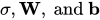 for the encoder.
Autoencoders are trained to minimize reconstruction errors (such as squared errors), often called the « loss »:

where is usually averaged over some input training set.
As mentioned earlier, autoencoder training is performed by backpropagation, just as in an ordinary feedforward neural network.
If the feature space  has a lower dimensionality than the input space
  , the feature vector
  can be regarded as a compressed representation of the input data
 . This is the case for an undercomplete autoassociator. If the hidden layers are larger than (overcomplete autoencoders), or equal to, the input layer, or the hidden units are given sufficient capacity, the autoencoder can potentially learn the identity function and become useless. However, experimental results have shown that in these cases autoencoders can still learn useful functions. [13] In the ideal case, one should be able to adapt the code dimensionality and the model capacity depending on the complexity of the data distribution being modeled. One way to do this is to use model variants known as regularized autoencoders.
There are various techniques for preventing autoencoders from learning the identity function and for improving their ability to capture important information and learn richer representations.
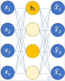
When representations are learned in a way that encourages sparsity, improved performance is achieved on classification tasks. A sparse autoencoder may include more (rather than fewer) hidden units than inputs, but only a small number of the hidden units are allowed to be active at the same time. This sparsity constraint forces the model to respond to the unique statistical features of the training data.
Specifically, a sparse autoencoder is an autoencoder whose training criterion includes a sparsity penalty on the code layer
  .
.

Recalling that  , the penalty encourages the model to activate (i.e., have an output value close to 1) certain areas of the network based on the input data, while deactivating all other neurons (i.e., have an output value close to 0).
This sparsity can be achieved by formulating the penalty terms in different ways.
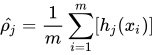
be the average activation of the hidden unit  (averaged over the
  training examples). The notation
 identifies the input value that triggered the activation. To encourage most of the neurons to be inactive,
 should be close to 0. Consequently, this method enforces the constraint
  where
where  is the sparsity parameter, a value close to zero. The penalty termtakes a form that penalizes for deviating significantly from , using the KL divergence:
 where sums over the
  hidden nodes in the hidden layer, and
  is the KL-divergence between a Bernoulli random variable with meanand a Bernoulli random variable with mean .
 .[18] For example, in the case of L1 the loss function takes the form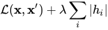
Denoising autoencoders (DAE) try to achieve a good representation by changing the reconstruction criterion.
Indeed, DAEs take a partially corrupted input and are trained to recover the original undistorted input. In practice, the objective of denoising autoencoders is to clean the corrupted input, or reduce noise. Two assumptions are inherent to this approach:
In other words, denoising is advocated as a training criterion for learning to extract useful features that will better represent the input at a higher level.
The training process of a DAE works as follows:
is corrupted into  through a stochastic mapping
 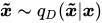 . is then mapped to a hidden representation using the same process as the standard autoencoder,
  .
. .
.The model's parameters  and
and  are trained to minimize the average reconstruction error over the training data, specifically, to minimize the difference between
  and the original uncorrupted input
  . Note that each time a random exampleis presented to the model, a new corrupted version is generated stochastically based on
  .
.
The above training process can be applied to any kind of corruption process. Some examples could be additive isotropic Gaussian noise, masking noise (a fraction of the input chosen at random for each example is forced to 0) or salt-and-pepper noise (a fraction of the input chosen at random for each example is set to its minimum or maximum value with uniform probability).
Corruption of the input is performed only during training. Once the model has learned the optimal parameters for extracting representations from the original data, no corruption is added.
The contractive autoencoder adds an explicit regularizer to its objective function that forces the model to learn an encoding that is robust to small variations in the input values. This regularizer corresponds to the Frobenius norm of the Jacobian matrix of the encoder activations with respect to the input. Since the penalty is applied only to training examples, this term forces the model to learn useful information about the training distribution. The final objective function has the following form:
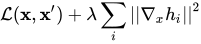
The autoencoder is called contractive because the CAE is encouraged to map a neighborhood of input points to a smaller neighborhood of output points.
DAE is connected to CAE: in the limit of small Gaussian input noise, DAEs make the reconstruction function resist small but finite input perturbations, while CAEs make the extracted features resist infinitesimal input perturbations.
A concrete autoencoder is a variant of the standard autoencoder architecture designed to select discrete features.[20] Unlike a standard autoencoder, which learns a latent representation that is a combination of potentially all the input features, a concrete autoencoder forces the latent space to consist of only a number of features specified by the user. The concrete autoencoder uses a continuous relaxation of the categorical distribution to allow gradients to pass through the feature-selector layer, which makes it possible to use standard backpropagation to learn the optimal subset of input features that minimize the reconstruction loss.
Variational autoencoders (VAEs) are generative models, similar to generative adversarial networks.[21] Their connection to this group of models stems mainly from the architectural similarity to the basic autoencoder (the final training objective includes an encoder and a decoder), but their mathematical formulation differs significantly. VAEs are directed probabilistic graphical models (DPGM) whose posterior is approximated by a neural network, forming an autoencoder-like architecture. Unlike discriminative modeling, which aims to learn a predictor given an observation, generative modeling tries to learn how the data is generated and to reflect the underlying causal relationships. Causal relationships have the potential for generalization.
Variational autoencoder models make strong assumptions regarding the distribution of latent variables. They use a variational approach for learning the latent representation, which results in an additional loss component and a specific estimator for the training algorithm called the Stochastic Gradient Variational Bayes (SGVB) estimator. It is assumed that the data is generated by a directed graphical model and that the encoder is learning an approximation
 to the posterior distribution
  where
where  and
and  denote the parameters of the encoder (recognition model) and decoder (generative model), respectively. The probability distribution of the VAE's latent vector typically matches that of the training data much more closely than in a standard autoencoder. The VAE objective has the following form:

Here,  denotes the Kullback–Leibler divergence. The prior over the latent variables is usually set to be the centered isotropic multivariate Gaussian
  ; however, alternative configurations have been considered.[24]
Typically, the shape of the variational distribution and the likelihood distribution is chosen so that they are factorized Gaussians:
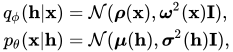
where  and
and  are the outputs of the encoder, and
  and
and  are the outputs of the decoder. This choice is justified by the simplifications[10],it produces when evaluating both the KL divergence and the likelihood term in the variational objective defined above.
VAEs have been criticized for generating blurry images.[25] The researchers using this model have shown, however, only the mean of the distributions,, rather than a sample of the learned Gaussian distribution
 .
.
It has been shown that these samples were too noisy due to the choice of a factorized Gaussian distribution.[25] [26] Using a Gaussian distribution with a full covariance matrix,

could solve this problem, but is computationally intractable and numerically unstable, since it requires estimating a covariance matrix from a single data sample. However, more recent research has shown that a restricted approach, where the inverse matrix , can rarely produce images with high-frequency detail.
Large-scale VAE models have been developed in various fields to represent data in a compact probabilistic latent space. For example, VQ-VAE[27] for image generation and Optimus for language modeling.
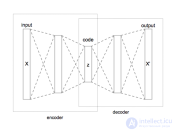
Autoencoders are often trained with a single-layer encoder and a single-layer decoder, but using deep (multilayer) encoders and decoders offers many advantages.
Geoffrey Hinton developed a technique for training multilayer deep autoencoders. His method involves treating each neighboring pair of layers as a restricted Boltzmann machine, so that pretraining approximates a good solution, followed by using backpropagation to fine-tune the results. This model became known as a deep belief network.
Researchers have debated whether joint training (i.e., training the entire architecture together with a single global reconstruction objective to optimize) would be better for deep autoencoders. A 2015 study showed that joint training learns better data models, as well as more representative features for classification, compared to the layer-wise method.[30] However, their experiments showed that the success of joint training depends heavily on the regularization strategies adopted.
Recently, autoencoders have seen little use for the «greedy» layer-wise pretraining of deep neural networks described above. After this method was proposed in 2006 by Geoffrey Hinton and Ruslan Salakhutdinov, it fairly quickly turned out that newer random-weight initialization methods were sufficient for further training of deep networks. Batch normalization, proposed in 2014, made it possible to train even deeper networks, while the residual-learning method proposed at the end of 2015 made it possible to train networks of arbitrary depth.
The main practical applications of autoencoders remain reducing noise in data, as well as reducing the dimensionality of high-dimensional data for visualization. With certain caveats regarding the dimensionality and sparsity of the data, autoencoders can yield projections of high-dimensional data that turn out to be better than those given by principal component analysis or by any other classical method.
Two main applications of autoencoders are dimensionality reduction and information retrieval , but modern variants have proven successful when applied to a variety of tasks.
Dimensionality reduction was one of the first applications of deep learning, and one of the early motivations for studying autoencoders. The task is to find a suitable projection method that maps data from a high-feature space to a low-feature space.
One of the important papers on this subject was Hinton's 2006 paper:[29] in that study, he pretrained a multilayer autoencoder using a stack of RBMs, and then used their weights to initialize a deep autoencoder with progressively decreasing hidden layers, down to a bottleneck of 30 neurons. The resulting 30-dimensional code gave a lower reconstruction error compared to the first 30 components of principal component analysis (PCA), and produced a representation that was qualitatively easier to interpret, clearly separating clusters of data.
Representing data in a lower-dimensional space can improve performance on tasks such as classification. Indeed, many forms of dimensionality reduction place semantically related examples close to one another, promoting generalization.
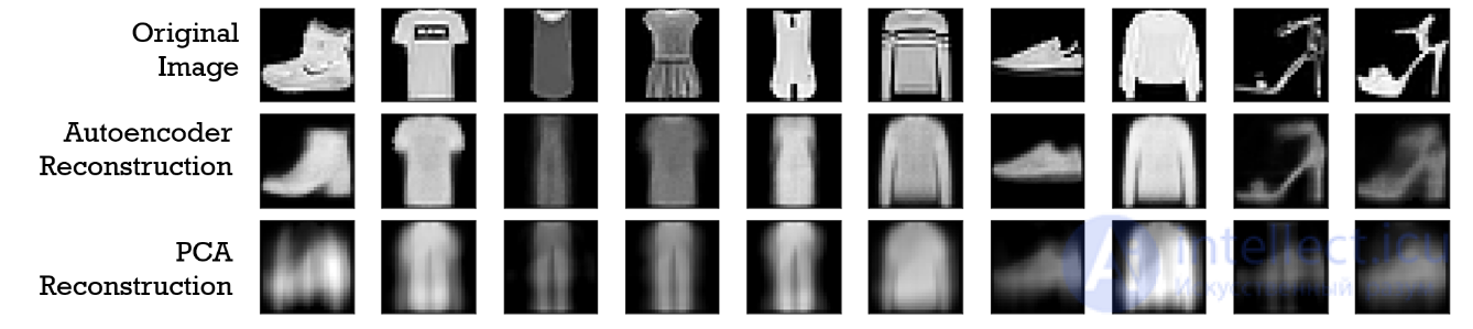
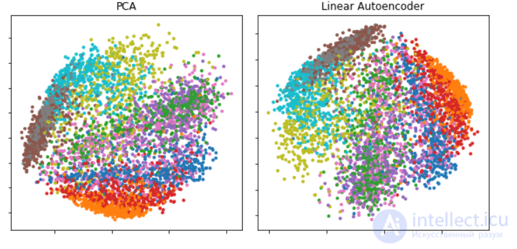
Reconstruction of 28x28 pixel images using an autoencoder with a code size of two (a two-dimensional hidden layer), and reconstruction from the first two principal components of PCA. The images are taken from the Fashion MNIST dataset.[32]
If linear activations are used, or only a single hidden sigmoid layer, then the optimal solution for an autoencoder is strongly related to principal component analysis (PCA). The weights of an autoencoder with a single hidden layer of size (where is smaller than the input size) span the same vector subspace as the first principal components, and the output of the autoencoder is an orthogonal projection onto this subspace. The autoencoder weights are not equal to the principal components, and are in general not orthogonal, yet the principal components can be recovered from them using singular value decomposition.
However, the potential of autoencoders lies in their non-linearity, which allows the model to learn more powerful generalizations compared to PCA, and to reconstruct the input with significantly less loss of information.
Information retrieval benefits particularly from dimensionality reduction, since search can become more efficient in certain types of low-dimensional spaces. Autoencoders have indeed been applied to semantic hashing, proposed by Salakhutdinov and Hinton in 2007. By training the algorithm to produce a low-dimensional binary code, all database entries can be stored in a hash table mapping binary code vectors to entries. This table would then support information retrieval, returning all entries with the same binary code as the query, or slightly less similar entries, by flipping a few bits of the query's encoding.
Another application of autoencoders is anomaly detection. By learning to replicate the most salient features of the training data under some of the constraints described earlier, the model is encouraged to learn to accurately reproduce the most frequently observed characteristics. When faced with anomalies, the model should degrade its reconstruction performance. In most cases, only data with normal instances is used to train the autoencoder; in other cases, the frequency of anomalies is small compared to the observation set, so that their contribution to the learned representation can be ignored. After training, the autoencoder will accurately reconstruct «normal» data, but will fail to do so with unfamiliar, anomalous data. The reconstruction error (the error between the original data and its low-dimensional reconstruction) is used as the anomaly score for anomaly detection.
However, recent literature has shown that some autoencoding models can, counterintuitively, be very good at reconstructing anomalous examples, and consequently fail to reliably perform anomaly detection.
The characteristics of autoencoders are useful in image processing.
One example can be found in lossy image compression, where autoencoders have outperformed other approaches and proved competitive with JPEG 2000.
Another useful application of autoencoders in image preprocessing is denoising.
Autoencoders have found applications in more complex contexts, such as medical imaging, where they have been used for image denoising ,as well as for super-resolution. In image-based diagnostics, experiments have applied autoencoders to detect breast cancer and to model the relationship between cognitive decline in Alzheimer's disease and the latent features of an autoencoder trained on MRI.
In 2019, molecules generated using variational autoencoders were validated experimentally in mice.
Recently, a stacked autoencoder framework produced promising results in predicting the popularity of social media posts, which is useful for online advertising strategies.
Autoencoders have been applied to machine translation, which is usually called neural machine translation (NMT). In NMT, texts are treated as sequences that must be encoded as part of the training procedure, while on the decoder side the target languages are generated. Language-specific autoencoders incorporate linguistic features into the training procedure, such as Chinese decomposition features.

Comments