
Lecture
In machine learning, knowledge distillation or model distillation — is the process of transferring knowledge from a large model to a smaller one. While large models (such as very deep neural networks or ensembles of many models) have greater knowledge capacity than small models, this capacity may not be fully utilized. Evaluating a model can be just as computationally expensive even if it uses only a small fraction of its knowledge capacity. Knowledge distillation transfers knowledge from a large model to a smaller one without loss of validity . Because smaller models are less costly to evaluate, they can be deployed on less powerful hardware (such as a mobile device ).
Model distillation should not be confused with model compression , which describes techniques for reducing the size of the large model itself without training a new model. Model compression typically preserves the architecture and the nominal number of parameters of the model while reducing the number of bits per parameter.
Knowledge extraction has been used successfully in several machine learning applications, such as object detection , acoustic models , and natural language processing . Recently it has also been introduced for building graph neural networks applicable to non-graph data.
Data distillation is needed for
Transferring knowledge from a large model to a small one must somehow train the latter without loss of validity. If both models are trained on the same data, the smaller model may not have enough capacity to learn a compact representation of knowledge compared to the large model. However, some information about the compact representation of knowledge is encoded in the pseudo-likelihoods assigned to its outputs: when the model correctly predicts a class, it assigns a large value to the output variable corresponding to that class, and smaller values to the other output variables. The distribution of values among the outputs for a given record provides information about how the large model represents knowledge. Consequently, the goal of economically deploying a valid model can be achieved by training only the large model on the data, taking advantage of its superior ability to learn compact representations of knowledge, and then distilling that knowledge into the smaller model by training it to learn the large model's soft output.
Diffusion models learn to generate data by reversing the diffusion process, i.e., the model learns to turn random noise into a coherent image (usually corresponding to a given prompt).
The problem here is the word gradually. This requires hundreds of steps, and each of them requires a large amount of computation.
Why do we do it this way? Well, we can't just jump from noise to a coherent image, that would lead to abstract, surreal results. Noise is random and does not contain an image as such (generally speaking). Gradually removing the noise allows the overall outline of the image to emerge, which can then be refined step by step, using the previous steps as a base. It's the same with people – you can't write an entire Python application in one go – you usually write the code piece by piece, and it kind of evolves.
But why do we need so many steps? Apparently, this is more a result of the initial mathematical description of the problem than anything else. It reminds me how often the formulation of a problem and the language used dictate the solution.
The idea here is that we don't do it the way described above. If you think about it, why do we need to predict every step ??. We can predict every other step, skipping a step both in training and in inference. The student no longer removes noise from a random noisy image. It removes noise from an image that has already been processed by the parent model, and the parent model is already trained and knows what it's doing (that's the benefit of teachers for you).
Thus, in the student model we will have half as many steps as in the parent model, and it turns out that the quality is almost exactly the same. We then take this student model and use it as a teacher, and create a new student model. We then train the new student using this new teacher model, and again during training try to predict only every other step, and so on. Eventually, we repeat this process many times, compressing the model and the number of steps, halving them each time. We keep doing this process until we are no longer satisfied with the results. In this way, we effectively cut the computational requirements in half with each distillation, and at this point it seems possible to have only four to six steps, with the model still performing just as well as the initial teacher model with hundreds of steps. This is called the distillation process.
Here is a diagram:
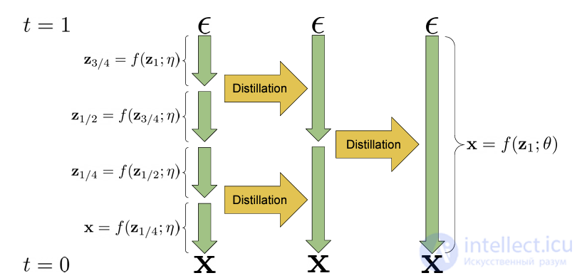
Distillation process
Visualization of two iterations of the progressive distillation algorithm. The sampler f(z; η), which maps random noise ε into samples x in 4 deterministic steps, is distilled into a new sampler f(z; θ), performing only one step.
This method makes it possible to train a compact model (student) based on a more complex and powerful model (teacher).
Example:
In computer vision, MobileNet can be trained using ResNet as the teacher model to achieve a good balance between quality and speed.
This method aims to reduce the amount of training data without loss of model quality.
Example:
In NLP, a small sample of texts can be generalized through GPT-based synthesized examples, preserving key semantic properties.
Given a large model as a function of a vector variable  , trained for a particular classification task, typically the last layer of the network is a softmax of the form
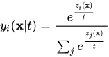
where  is the temperature , a parameter that for standard softmax equals 1. The softmax operator converts the logit values
  into pseudo-probabilities: higher temperature values generate softer distributions of pseudo-probabilities among the output classes. Knowledge distillation consists of training a smaller network, called the distilled model , on a dataset called the transfer set (which differs from the dataset used to train the large model), using cross-entropy as the loss function between the outputs of the distilled model
  and the output of the large model
  on the same record (or the average of individual outputs, if the large model is an ensemble), using a high softmax temperature valueTfor both models

In this context, a high temperature increases the entropy of the outputs, thereby providing more information for training the distilled model compared with hard targets, while at the same time reducing the variance of the gradient between different records, thereby enabling a higher learning rate .
If ground-truth data is available for the transfer set, the process can be strengthened by adding to the loss the cross-entropy between the outputs of the distilled model (computed with  ), and the known label

where the loss component with respect to the large model is weighted by a coefficientT2 since, as the temperature increases, the gradient of the loss with respect to the model weights increases by a factor of
  .
.
Provided that the logits have zero mean , it can be shown that model compression is a special case of knowledge distillation. The gradient of the knowledge-distillation loss  with respect to the logit of the distilled model
  is given by
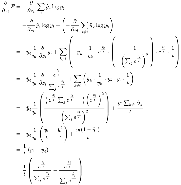
wherez_i are the logits of the large model. For large values ofTthis can be approximated as
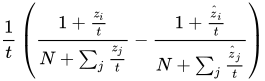
and under the zero-mean hypothesis 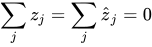 this becomes
  , which is the derivative of
  , i.e., the loss is equivalent to matching the logarithms of the two models, as is done in model compression.
The Optimal Brain Damage (OBD) algorithm is as follows:
Repeat until the desired level of sparsity or performance is achieved:
Train the network (using methods such as backpropagation) until a reasonable solution is obtained.
Compute the saliency for each parameter
Delete some of the least significant parameters
Deleting a parameter means fixing the parameter at zero. «Saliency» of a parameter  is defined as
  , where
  is the loss function.
The second derivative  can be computed using the second-order backpropagation method .
The idea of Optimal Brain Damage is to approximate the loss function in the neighborhood of the optimal parameter.  by a Taylor expansion:
  where
where  , with being optimal, and the cross derivatives
  are ignored to save computation.
Thus, the saliency of a parameter approximates the increase in loss if that parameter is removed.
A related methodology was model compression or pruning, in which a trained network was reduced in size. This was first done in 1965 by Alexey Ivakhnenko and Valentin Lapa (Ukraine) (1965). Their deep networks were trained layer by layer using regression analysis. Redundant hidden units were pruned using a separate validation set. Other methods for compressing neural networks include Biased Weight Decay and Optimal Brain Damage.
An early example of neural network distillation was published by Jürgen Schmidhuber in 1991 in the field of recurrent neural networks (RNNs). The problem was sequence prediction for long sequences, i.e., deep learning . It was solved using two RNNs. One of them ( the automatizer ) predicted the sequence, while the other ( the chunker ) predicted the automatizer's errors. At the same time, the automatizer predicted the internal states of the chunker. Once the automatizer managed to predict the chunker's internal states well, it began correcting the errors, and the chunker soon became obsolete, leaving only a single RNN in the end.
The idea of using the output of one neural network to train another neural network was also studied as a teacher-student network configuration. In 1992, several papers studied the statistical mechanics of teacher-student configurations with committee machines or both machines with parity.
The compression of the knowledge of several models into a single neural network in 2006 was called model compression : compression was achieved by training a smaller model on large amounts of pseudo-data labeled by the higher-performing ensemble, optimizing so that the logit of the compressed model matches the logit of the ensemble. In the preprint on knowledge extraction by Geoffrey Hinton et al. (2015), the concept was formulated and some results achieved on the image classification task were shown.
Knowledge distillation is also related to the concept of behavioral cloning, discussed by Faraz Torabi et al.
Model and data distillation — are powerful techniques for creating more compact, faster, and more efficient machine learning systems, especially relevant for mobile devices, IoT, and cloud services.

Comments