
Lecture
The Hopfield network (Hopfield network) — a fully connected neural network with a symmetric weight matrix. During operation, the dynamics of such networks converge to one of a set of equilibrium states. These equilibrium states are determined in advance during training; they are local minima of a functional called the network energy (in the simplest case — local minima of a negative-definite quadratic form on an n-dimensional cube). Such a network can be used as autoassociative memory, as a filter, and also for solving certain optimization problems. Unlike many neural networks, which operate until they produce an answer after a fixed number of steps, Hopfield networks operate until equilibrium is reached, when the next state of the network is exactly equal to the previous one: the initial state is the input pattern, and at equilibrium the output pattern is obtained .
A variation of it is the Hamming network.
The Hopfield neural network with double-threshold neurons or neurons with a step response has attracted considerable interest as a method for solving difficult optimization problems [8, 9]. Takefuji and Lee proposed a two-state (binary) hysteresis threshold model to suppress oscillatory behavior in the dynamics of Hopfield neural networks [10]. However, Tatemi and Tamura showed that the Takefuji and Lee model did not always guarantee a decrease in the energy function [11]. Wang also explained why the model could lead to inaccurate results and oscillatory behavior during the convergence process [12]. Following their reports, several modifications of the hysteresis function were proposed, such as the binary version by Galan and Muñoz [13] and the multivalued version by Bhartikar and Mendel [14]. Smith and Portman showed that the simple «neural» optimization networks described by Tank and Hopfield were equivalent to a circuit containing Schmitt triggers with variable thresholds, and that the hysteresis of the Schmitt triggers played a major role in determining stability [15, 16]. The architecture
of the Hopfield neural network has also been applied to real-time control of
crossbar switches used for switching high-speed
packets at maximum throughput, and it has been
shown to achieve very good performance, especially
for small-scale crossbar switch problems [17-21].
In the paper «Binary Hopfield Neural Network with
Hysteresis for Large Crossbar Packet Switches» by
the authors Guangpu Xia, Zheng Tang, Yong Li, and
Jiahai Wang, a new Hopfield neural network
architecture was presented for efficiently solving
the crossbar switch problem. Unlike the original
Hopfield neural network, the proposed architecture
uses hysteresis binary neurons. It was theoretically
proven that the Hopfield neural network architecture
with hysteresis binary neurons converges just like
the original Hopfield neural network. To see how well
the Hopfield neural network architecture with
hysteresis binary neurons handles solving the
crossbar switch problem, a large number of computer
simulations were performed. The simulation results
show that the Hopfield neural network architecture
with hysteresis binary neurons is much better than
previous works, including the Hopfield neural network
architecture, the Traudet architecture, and the maximum neural network for the crossbar switch problem, as with the original Hopfield neural network, both with respect to computation time and solution quality. The total input to neuron i of the Hopfield neural network with hysteresis binary neurons is

where
 is the total input of neuron i;
 – the output of neuron j;
 – the strength of the symmetric connection from neuron j to neuron i;
 – is the compensating bias of neuron i.
Each neuron computes its output from its input. However, unlike
the neurons of the Hopfield neural network with a two-state threshold (Figure
1.5(a)), hysteresis binary neurons either change the value of their output or
leave it unchanged according to the hysteresis threshold rule (Figure
1.5(b)):

where a – is the upper trip point (UTP); b – is the lower trip point (LTP). As shown in Figure 1.5(b),
if  , and if ,
  then = .
When  is held unchanged, i.e.
  if the previous value was
  1, and
  if the previous value was 0.
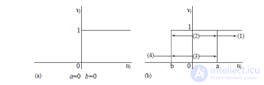
Figure 1.5 – Activation functions: a) threshold; b) hysteresis
Consider the energy

If wij = wji and wii = 0; the change ΔE in the energy E due to
the changing state of neuron i from  is
is
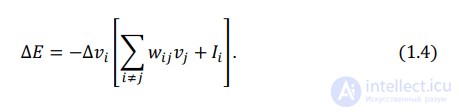
Using Equation 1.1 we have:

There are two types of changes in the state of the i-th neuron, caused by
adjusting Equation 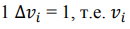 , i.e. it changes from 0 to 1.
According to the hysteresis threshold rule (Equation 1.2), when  changes from 0 to 1, we have that
  .
.
Then 
thus, the energy is guaranteed to decrease if a > 0.
From the hysteresis threshold rule (Equation 1.2), when it changes from 1
to 0, we have that  . Then

thus, the energy is guaranteed to decrease if b ≤ 0.
Hence, convergence of the energy function to a
local/global minimum is always guaranteed only if  and b ≤ 0.
Note that the theoretical results presented an extract for the original Hopfield neural network, while the original
network is only one special case at a = b = 0.
Moreover, when  and b ≤ 0, the absolute value of the energy decrease
  is greater than or at least the same as that of the original network at each update, and thus the network with hysteresis binary neurons converges to a stable state faster than the original network.
Furthermore, although the results presented are theoretical excerpts for the unidirectional Hopfield neural network, they can easily be extended to
bidirectional or even multidirectional Hopfield neural networks.
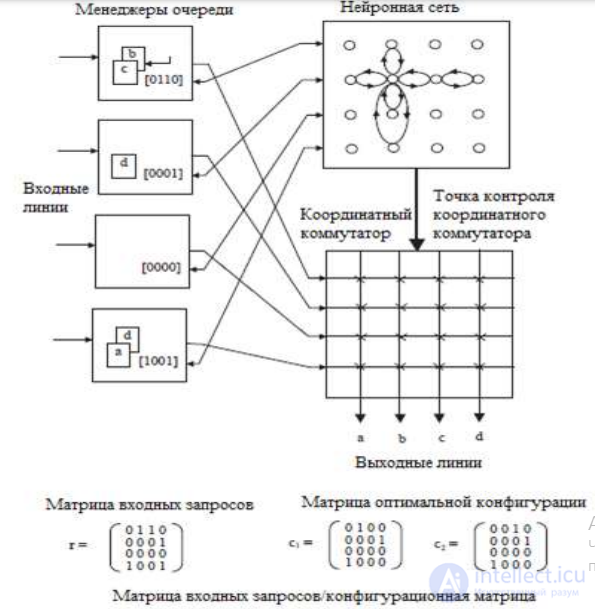
Figure 1.6 – Schematic control architecture of a 4 x 4 crossbar switch


Comments