
Lecture
Recursion is the property of an object to imitate itself. An object is recursive if its parts look the same as the whole object. Recursion is very widely used in mathematics and programming:
This article is devoted to analyzing the complexity of recursive algorithms; it provides the necessary mathematical background and examines examples. It also describes the possibility of replacing recursion with a loop, and tail recursion.
A recursive algorithm always breaks a problem down into parts that are structurally the same as the original problem, but simpler. To solve the subproblems, the function is called recursively, and their results are combined in some way. The problem is divided only when it cannot be solved directly (i.e., it is too complex).
For example, the task of processing an array can often be reduced to processing its parts. Division into parts is performed until they become elementary, i.e., simple enough to obtain a result without further simplification.
The algorithm divides the original array into two parts — the first element and the array of the remaining elements. Two simple cases are distinguished when no division is required — all elements have been processed, or the first element is the one being sought.
In the search algorithm, the array could be divided differently (for example, in half), but this would not affect efficiency. If the array is sorted, then dividing it in half is worthwhile, since at each step the amount of data to be processed can be reduced by half.
Binary search is performed on a sorted array. At each step, the element being sought is compared with the value located in the middle of the array. Depending on the result of the comparison, either the left or the right part can be «discarded».
Fibonacci numbers are defined by a recurrence relation, that is, one in which the value of an element is expressed in terms of previous elements: F0=0,F1=1,Fn=Fn−1+Fn−2,n>2.
At each step, the quicksort algorithm selects one of the elements (the pivot) and, relative to it, divides the array into two parts, which are processed recursively. Elements smaller than the pivot are placed in one part, and the rest in the other.
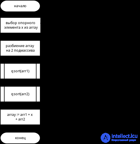
Flowchart of the quicksort algorithm
The merge sort algorithm is based on the ability to quickly merge sorted arrays (or lists) so that the result remains sorted. The algorithm divides the original array into two parts in an arbitrary way (usually in half), recursively sorts them, and merges the result. The division continues as long as the array size is greater than one, since an empty array and an array of a single element are always sorted.
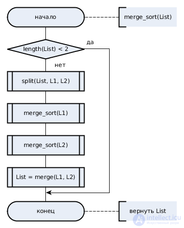
Flowchart of merge sort
At each step of the merge, the first unprocessed element is selected from both lists. The elements are compared, the smaller one is added to the result and marked as processed. Merging continues until one of the lists becomes empty.
When analyzing the complexity of iterative algorithms, the cost of iterations and their number are calculated for the worst, best, and average cases . However, this approach cannot be applied to a recursive function, since it results in a recurrence relation. For example, for a function that searches for an element in an array:

Recurrence relations do not allow us to evaluate complexity directly — we cannot simply compare them, and therefore cannot compare the efficiency of the corresponding algorithms. It is necessary to obtain a formula that describes the recurrence relation — a universal way to do this is to select a formula using the substitution method, and then prove that the formula corresponds to the relation using the method of mathematical induction.
This consists of successively replacing the recurrent part in the expression to obtain new expressions. The replacement is carried out until it becomes possible to grasp the general principle and express it as a non-recurrent formula. For example, for searching for an element in an array:

We have derived a formula; however, the first step contains an assumption, i.e., there is no proof that the formula corresponds to the recurrent expression — obtaining a proof is made possible by the method of mathematical induction.
Allows one to prove the truth of some statement (Pn), and consists of two steps:
Let us prove the correctness of the assumption made when estimating the cost of the search function
(  =(n+1)×O(1)):
 =2×O(1) is true from the condition (it can be substituted into the original recurrence formula);
 =(n+1)×O(1);
 =((n+1)+1)×O(1)=(n+2)×O(1);
 =O(1)+(n+1)×O(1)=(n+2)×O(1);
the statement is proved.
Often, such a proof is a fairly labor-intensive process, but it is even harder to identify the pattern using the substitution method. For this reason, the so-called general method is used .
The general method is not universal; for example, it cannot be used to estimate the complexity of the Fibonacci number computation algorithm given above. However, it is applicable to all cases that use the «divide and conquer» approach :

Equations of this form arise when the original problem is divided into a subproblems, each of which processes nb elements. fn — the cost of the operations of splitting the problem into parts and combining the solutions. In addition to the form of the relation, the general method imposes restrictions on the function fn, distinguishing three cases:

The validity of the statements for each case has been proved formally . The task of analyzing a recursive algorithm is now reduced to determining which case of the master theorem corresponds to the recurrence relation.
The algorithm splits the input data into 2 parts (b = 2), but processes only one of them (a = 1), 
. The function for splitting the problem and combining the result grows at the same rate as  which means the second case of the theorem must be used:

The recursive function divides the original problem into one subproblem (a = 1); the data is divided into one part (b = 1). We cannot use the master theorem to analyze this algorithm, since the condition b>1 is not satisfied.
To carry out the analysis, the substitution method can be used, or the following reasoning: each recursive call reduces the dimensionality of the input data by one, meaning there will be n of them in total, each of which has a complexity of
O(1). Then

The input data is divided into two parts, both of which are processed: 
When processing a list, splitting may require Θ(n) operations, while for an array it is performed in constant time (Θ(1)). However, combining the results will in any case take Θ(n), so fn=n.
The second case of the theorem is used: 
In the best case, the original array is split into two parts, each containing half of the original data. Splitting requires n operations. The complexity of assembling the result depends on the data structures used — for an array, O(n), for a linked list, O(1). a=2,b=2,fn=b, which means the complexity of the algorithm will be the same as that of merge sort: TquickSortn=O(n⋅logn).
However, in the worst case, the minimum or maximum element of the array will constantly be chosen as the pivot. Then b=1, which means we again cannot use the master theorem. However, we know that in this case n recursive calls will be made, each of which performs a split of the array into parts (O(n)) — which means the complexity of the algorithm is TquickSortn=O(n2).
When analyzing quicksort using the substitution method, the best and worst cases would also have to be considered separately.
Analyzing the time complexity of recursive functions is considerably more difficult than the corresponding evaluation of loops, but the main reason loops are preferable is the high cost of a function call.
After a call, control is transferred to another function. To transfer control it is enough to change the value of the program counter register, in which the processor stores the number of the currently executing instruction — control is transferred to branches of an algorithm in the same way, for example, when using a conditional statement. However, a call is not merely a transfer of control, since after the called function finishes its computations, it must return control to the point from which the call was made, and also restore the values of the local variables that existed there before the call.
To implement this behavior a stack (call stack) is used — the instruction number for the return and information about local variables are placed on it. The stack is not infinite, so recursive algorithms can cause it to overflow, and in any case working with it can take up a significant amount of time.
In a number of cases a recursive function can quite easily be replaced by a loop, for example, the search and binary search algorithms discussed above . In some cases a more creative approach is required, but most often such a replacement turns out to be possible. In addition, there is a special kind of recursion in which the recursive call is the last operation performed by the function. Obviously, in such a case the calling function will not in any way modify the result, which means there is no point in it returning control. Such recursion is called tail recursion — compilers automatically replace it with a loop.
Making recursion tail recursion is often facilitated by the accumulator parameter method , which consists of adding an extra accumulator argument to the function, in which the result is accumulated. The function performs computations with the accumulator before the recursive call. A good example of using this technique is the function for computing a factorial:
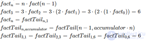
As a more complex example, let us consider the function for computing Fibonacci numbers. The main function calls an auxiliary one, which uses the accumulator parameter method, passing as arguments the initial value of the iterator and two accumulators (the two previous Fibonacci numbers).
The function with the accumulator parameter returns the accumulated result if the specified number of numbers has been calculated; otherwise it increments the counter, calculates a new Fibonacci number, and makes a recursive call. Optimizing compilers can detect that the result of the function call is passed unchanged to the function's output and replace it with a loop. This technique is especially relevant in functional and logic programming languages, since in them the programmer cannot explicitly use loop constructs.

Comments