
Lecture
Algorithm (Latin algorithmi — from the name of the mathematician Al-Khwarizmi) — is a finite set of precisely defined rules for solving an arbitrary class of problems, or a set of instructions describing the sequence of actions of an executor for solving a certain problem. In the older interpretation, the word "sequence" was used instead of "order," but as parallelism developed in the operation of computers, the word "sequence" began to be replaced by the more general word "order." Independent instructions can be executed in an arbitrary order, in parallel, if the executors being used allow it.
Earlier in the Russian language, the word was written as "algorifm," and although this spelling is rarely used now, there is nonetheless an exception (Markov's normal algorifm).
Meta-algorithm (Metaalgorithm) is a generalization of the concept of an algorithm. Classical formalizations of the concept of an algorithm (for example, normal algorithms) do not fully provide an adequate formalization of the intuitive notion of an algorithm. Normal algorithms, for instance, do not provide for the unambiguous application of a normal algorithm to itself (since applying an algorithm to a scheme of an algorithm requires converting the algorithm scheme into some word in the alphabet used, which can only be done "manually," based on certain conventions; since conventions are nothing more than agreements, they can change, which entails ambiguity in applying the algorithm to itself). A certain modification of normal algorithms provides for the unambiguous application of such algorithms to themselves. This formalization of the concept of an algorithm is considered to be the definition of a meta-algorithm
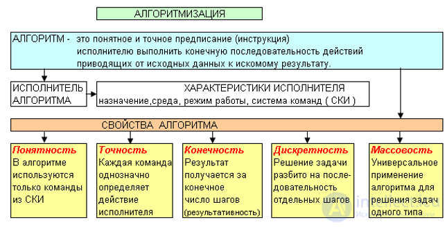
A computer often serves as the executor, but the concept of an algorithm does not necessarily apply only to computer programs; for example, a clearly described recipe for preparing a dish is also an algorithm, in which case the executor is a person (or possibly some mechanism, a weaving loom, etc.).
Algorithms can be divided into computational ones (which will mostly be discussed below) and control algorithms. Computational algorithms essentially transform certain initial data into output, thereby implementing the computation of some function. The semantics of control algorithms can differ substantially and come down to issuing the necessary control actions either at set moments in time or in response to external events (in this case, unlike a computational algorithm, a control algorithm can remain correct under infinite execution).
The concept of an algorithm belongs to the initial, fundamental, basic concepts of mathematics. Computational processes of an algorithmic nature (arithmetic operations on integers, finding the greatest common divisor of two numbers, and so on) have been known to humanity since ancient times. However, the concept of an algorithm took explicit shape only at the beginning of the 20th century.
The partial formalization of the concept of an algorithm began with attempts to solve the decision problem (German: Entscheidungsproblem), which was formulated by David Hilbert in 1928. The subsequent stages of formalization were necessary for defining effective computations, or the "effective method"; among such formalizations are the recursive functions of Gödel — Herbrand — Kleene of 1930, 1934, and 1935, Alonzo Church's λ-calculus of 1936, Emil Post's "Formulation 1" of 1936, and the Turing machine.
" We rarely fully understand what we actually want. "
François de La Rochefoucauld
" An algorithm must be stated in such a way that it will get executed by a computer. "
Donald E. Knuth
The maxim of the Duke de La Rochefoucauld quoted above makes one cautious about attempting to briefly characterize the course being offered to you. What should it be called?
The range of topics we are about to address is assigned by numerous textbooks to such branches of science as theoretical computer science, finite mathematics, discrete mathematics, and others. The authority of the "Mathematical Encyclopedia" (Moscow, 1977–1985) does not help: the problems of classification remain even after consulting its dictionary entries. Strangely enough, these entries — on closely related topics — were written by different specialists who did not coordinate their interpretations of the concepts being defined.
Not finding the support he expected, the author risked ending up in almost the same position as the American logician Raymond M. Smullyan, who never did come up with a title for his well-known book. Still, help arrived — from two Frenchmen, Patrice Naudin and Claude Quitte. After a fortunate encounter with their hefty volume "Algorithmic Algebra" (Moscow, 1999), no similar word combinations seem too bold anymore. So I suggest the reader regard our course as an introduction to computer algorithmics.
The subject of discussion will of course be algorithms, and it would be convenient to begin with a formal definition of this concept. But doing so is by no means simple: one would need to delve into the content of the highly nontrivial theory of algorithms, which can hardly be considered introductory material.
Can one manage without a definition, relying solely on the reader's intuitive notion of the essence of an algorithm? Perhaps what is concerning is the excessive popularity of the term in question and, as is said in such cases, its overly broad interpretation. Thus, the author has come across "the chess player's algorithm" (in a book), "the algorithm for gathering information" in a sociological survey (in a newspaper publication), and others.
Therefore, let us take as a basis the notion of an algorithm as a description of some computational process, and then introduce certain refinements. Nevertheless, our illustrations will often be examples of a non-computational nature, not directly related to computer information processing, for which I hope the reader will not judge us.
First, some terminological clarifications. Often, for the sake of brevity, we will replace the phrase "description of a computational process" with the short word "process," which should not mislead the reader. Indeed, we will more often merely be constructing algorithms, without any intention of applying them right away. Moreover, if an algorithm is a description of a process, then a method of representing an algorithm is a "description of a description of a process." One is tempted to drop half of the "descriptions."
So, let us agree that the form of writing an algorithm — its format and its content — is by no means arbitrary, but is subject to quite definite constraints.
Let us begin with the formats for writing algorithms, of which quite a few are known. A reader familiar with programming technology follows fairly rigid rules of a specific language when writing an algorithm — it does not matter which one. It is quite likely that his first lessons were devoted to the flowchart language. Another variety of diagram language is represented by the very compact Nassi–Shneiderman diagrams. Both graphical formats have their advantages and disadvantages, but this is not the place to discuss them. What is common to all graphical formats is the ability either to place the descriptive text inside the blocks or to place the commentary outside the drawing.
Given the wide variety of ways to write an algorithm, we give preference to the "primary" form, namely, the verbal description. Of course, in this variant one also resorts to a number of notations, usually quite obvious, in particular, the explicit numbering of steps. An alternative to excessive brevity can be additional comments.

A page from the "Algebra" of Al-Khwarizmi — a mathematician from Khwarezm, whose name gave rise to the word algorithm.
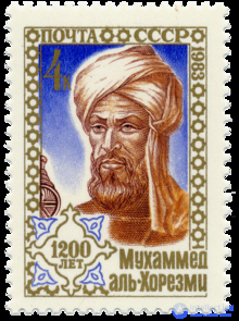
Al-Khwarizmi on a Soviet postage stamp
The modern formal definition of a computational algorithm was given in the 1930s—1950s in the works of Turing, Post, Church (the Church–Turing thesis), N. Wiener, and A. A. Markov.
The word «algorithm» itself derives from the name of the Khwarezmian scholar al-Khwarizmi. Around 825 he wrote the treatise Kitab al-jabr wal-muqabala («The Compendious Book on Calculation by Completion and Balancing»), from whose original title the word «algebra» derives (al-jabr — restoration). In this book he gave the first description of the positional decimal number system invented in India. The Persian original of the book has not survived. Al-Khwarizmi formulated the rules of calculation in the new system and was probably the first to use the digit 0 to denote a missing position in the notation of a number (its Indian name was translated by the Arabs as as-sifr, or simply sifr, from which come such words as «cipher» and «zero»). Around the same time, Indian numerals also began to be adopted by other Arab scholars.
In the first half of the twelfth century, al-Khwarizmi's book, in Latin translation, made its way into Europe. The translator, whose name has not come down to us, gave it the title Algoritmi de numero Indorum («Al-Khwarizmi on the Hindu Art of Reckoning») — thus the Latinized name of the Central Asian scholar was placed in the title of the book. Today it is believed that the word «algorithm» entered the European languages precisely through this translation. Over the following centuries many other works appeared devoted to the same subject — teaching the art of calculation with numerals — and all of them contained the word algoritmi or algorismi in their title.
Later authors knew nothing about al-Khwarizmi himself, but since the first translation of the book begins with the words: «Dixit algorizmi: …» («Al-Khwarizmi said: …»), the word continued to be associated with the name of a specific person. A very widespread version held that the book was of Greek origin. In a thirteenth-century Anglo-Norman manuscript, written in verse, we read:
Algorism was invented in Greece.
It is a part of arithmetic. It was invented by a master named Algorism, who gave it his own name. And since he was called Algorism,
He named his book «Algorism».
Around 1250, the English astronomer and mathematician John of Sacrobosco wrote a treatise on arithmetic, Algorismus vulgaris, which for centuries became the standard textbook on calculation in the decimal positional system at many European universities. In the introduction, Sacrobosco named as the author of the science of reckoning a sage called Algus (Algus). And in the popular medieval poem «Roman de la Rose» (1275—1280) by Jean de Meun, the «Greek philosopher Algus» is placed alongside Plato, Aristotle, Euclid, and Ptolemy! A variant spelling of the name, Argus (Argus), was also encountered. And although, according to ancient Greek mythology, the ship «Argo» was built by Jason, it was this Argus who was credited with building the ship.
«Master Algus» (or Argus) became, in medieval literature, the personification of the art of reckoning. Both in the already-mentioned «Roman de la Rose» and in the well-known Italian poem «Il Fiore», written by Durante, there are passages stating that even «mestre Argus» would not be able to count how many times lovers quarrel and reconcile. The English poet Geoffrey Chaucer, in the poem «The Book of the Duchess» (1369), writes that even the «noble countour Argus» would not be able to count the monsters that appeared to the hero in his nightmarish visions.
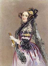
Baroness Ada Lovelace, who is considered the first programmer.
Over time, however, such explanations occupied mathematicians less and less, and the word algorism (or algorismus), which invariably appeared in the titles of mathematical works, came to mean a method of performing arithmetic operations by means of Arabic numerals, that is, on paper, without the use of an abacus. It was in this sense that it entered many European languages. For example, marked as «archaic», it appears in the authoritative English dictionary Webster’s New World Dictionary, published in 1957. The Brockhaus and Efron Encyclopedic Dictionary offers this interpretation: algorifm (incidentally, before the revolution the spelling algorifm, with the letter fita, was used) is derived «from the Arabic word Al-Goretm, meaning root».
An algorithm is the art of reckoning with numerals, but at first the word «cipher» referred only to zero. The famous French trouvère Gautier de Coincy (1177—1236) used the words algorismus-cipher (meaning the digit 0) in one of his poems as a metaphor to describe an utterly worthless person. Clearly, understanding such an image required appropriate preparation on the part of the audience, which means the new number system was already fairly well known to them.
For many centuries the abacus was in fact the only means of practical calculation, used by merchants, moneychangers, and scholars alike. The merits of calculation on the counting board were expounded in his writings by such an outstanding thinker as Gerbert of Aurillac (938—1003), who became Pope in 999 under the name Sylvester II. The new method made its way forward only with great difficulty, and the history of mathematics records the stubborn opposition between the camps of the algorists and the abacists (sometimes called Gerbertists), who advocated the use of the abacus for calculations instead of Arabic numerals. Interestingly, the famous French mathematician Nicolas Chuquet (1445—1488) was entered in the taxpayer register of the city of Lyon as an algorist (algoriste). But more than one century passed before the new method of reckoning was finally established — that much time was needed to work out generally accepted notation and to refine and adapt the methods of calculation for writing on paper. In Western Europe, teachers of arithmetic continued to be called «masters of the abacus» right up until the seventeenth century, as, for example, the mathematician Niccolò Tartaglia (1500—1557).
Thus, works on the art of reckoning were called Algorithms. Among the many hundreds, one can single out such unusual examples as the treatise written in verse, Carmen de Algorismo (the Latin carmen means verse), by Alexander de Villa Dei (died 1240), or the textbook by the Viennese astronomer and mathematician Georg Peurbach (1423—1461), Opus algorismi jocundissimi («The Most Delightful Work on Algorithm»).
Gradually the meaning of the word expanded. Scholars began to apply it not only to purely computational matters but also to other mathematical procedures. For example, around 1360, the French philosopher Nicole Oresme (1323/25–1382) wrote the mathematical treatise Algorismus proportionum («Calculation of Proportions»), in which he used, for the first time, powers with fractional exponents and in fact came very close to the idea of logarithms. When the so-called reckoning on lines replaced the abacus, the numerous manuals devoted to it came to be called Algorithmus linealis, that is, the rules of reckoning on lines.
It is worth noting that the original form algorismi lost its final letter after some time, and the word acquired the form algorism, more convenient for European pronunciation. Later this word, too, was corrupted in turn, most likely under the influence of the word arithmetic.
In 1684, Gottfried Leibniz, in his work Nova Methodvs pro maximis et minimis, itemque tangentibus…, was the first to use the word «algorithm» (Algorithmo) in an even broader sense: as a systematic method of solving problems of differential calculus.
In the eighteenth century, one of the German mathematical dictionaries, the Vollstandiges mathematisches Lexicon (published in Leipzig in 1747), still explained the term algorithmus as the concept of the four arithmetic operations. But this was not the only meaning, since the terminology of mathematical science was still only taking shape at the time. In particular, the expression algorithmus infinitesimalis was applied to methods of performing operations with infinitesimal quantities. Leonhard Euler also used the word algorithm; one of his works is titled precisely «On the Use of a New Algorithm for Solving the Pell Problem» (De usu novi algorithmi in problemate Pelliano solvendo). We can see that Euler's understanding of algorithm as a synonym for a method of solving a problem is already very close to the modern one.
However, almost two more centuries were needed before all the old meanings of the word fell out of use. This process can be traced through the example of the word «algorithm» entering the Russian language.
Historians date one of the surviving copies of the Old Russian arithmetic textbook known as «Schetnaya Mudrost» (Counting Wisdom) to 1691. This work is known in many variants (the earliest of them are almost a hundred years older) and traces back to even older manuscripts of the 16th century. From them one can trace how knowledge of Arabic numerals and the rules for operating with them gradually spread across Rus. The full title of this textbook is «This book, called in Hellenic and Greek arithmetica, in German algorisma, and in Russian numerical counting wisdom».
Thus, the word «algorithm» was understood by the first Russian mathematicians in the same way as in Western Europe. However, it was absent both from the famous dictionary of V. I. Dal and, a hundred years later, from the «Explanatory Dictionary of the Russian Language» edited by D. N. Ushakov (1935). Yet the word «algorifm» can be found both in the popular pre-revolutionary Encyclopedic Dictionary of the Granat brothers and in the first edition of the Great Soviet Encyclopedia (GSE), published in 1926. In both, it is interpreted in the same way: as a rule by which one of the four arithmetic operations is performed in the decimal number system. However, by the beginning of the 20th century, for mathematicians the word «algorithm» already meant any arithmetic or algebraic process carried out according to strictly defined rules, and this explanation is also given in subsequent editions of the GSE.
Algorithms increasingly became the subject of scholarly attention, and gradually this concept took one of the central places in modern mathematics. As for people far removed from mathematics, by the early 1940s they might have heard this word only during their schooling, in the phrase «Euclid's algorithm». Despite this, the algorithm was still perceived as a strictly specialized term, which is confirmed by the absence of corresponding entries in less voluminous publications. In particular, it is not even found in the ten-volume Small Soviet Encyclopedia (1957), let alone in single-volume encyclopedic dictionaries. But ten years later, in the third edition of the Great Soviet Encyclopedia (1969), the algorithm was already characterized as one of the fundamental categories of mathematics, «lacking a formal definition in terms of simpler concepts, and abstracted directly from experience». As we can see, the difference from the treatment in even the first edition of the GSE is striking! In forty years the algorithm turned into one of the key concepts of mathematics, and recognition of this came with the inclusion of the word no longer only in encyclopedias, but in dictionaries as well. For example, it appears in the academic «Dictionary of the Russian Language» (1981) precisely as a term from the field of mathematics.
Along with the development of the concept of the algorithm, its expansion from pure mathematics into other spheres gradually took place. This expansion was launched by the advent of computers, thanks to which the word «algorithm» entered all school computer science textbooks in 1985 and acquired new life. In general, one can say that its present-day fame is directly linked to the extent of computer proliferation. For example, in the third volume of the «Children's Encyclopedia» (1959), a good deal is said about computing machines, but they had not yet become something familiar and were perceived rather as an attribute of a bright but fairly distant future. Accordingly, algorithms are not mentioned once on its pages. But already in the early 1970s, when computers ceased to be an exotic curiosity, the word «algorithm» rapidly came into common use. Encyclopedic publications sensitively registered this. In the «Encyclopedia of Cybernetics» (1974), in the entry «Algorithm», it is already linked to implementation on computing machines, while the «Soviet Military Encyclopedia» (1976) even features a separate entry «Algorithm for Solving a Problem on a Computer». Over the past decade and a half or two, the computer has become an inseparable part of our lives, and computer terminology has become ever more familiar. The word «algorithm» is probably known to everyone nowadays. It has confidently stepped even into colloquial speech, and today we often encounter in newspapers and hear in politicians' speeches expressions such as «algorithm of behavior», «algorithm of success», or even «algorithm of betrayal». Academician N. N. Moiseev named his book «Algorithms of Development», while the well-known physician N. M. Amosov titled his — «Algorithm of Health» and «Algorithms of the Mind». This means that the word lives on, enriched with ever new meanings and shades of sense.
Various definitions of the algorithm, explicitly or implicitly, contain the following set of common requirements:
Various theoretical problems of mathematics and the acceleration of the development of physics and technology placed on the agenda the need for a precise definition of the concept of the algorithm.
The first attempts to clarify the concept of the algorithm and to investigate it were undertaken in the first half of the 20th century by Alan Turing, Emil Post, Jacques Herbrand, Kurt Godel, A. A. Markov, and Alonzo Church. Several definitions of the concept of the algorithm were developed, but it was subsequently found that they all define the same concept (see the Church–Turing thesis)
The Russian mathematician V. A. Uspensky, founder of structural linguistics in the Soviet Union, believed that the concept of the algorithm first appeared with Emile Borel in 1912, in an article on the definite integral. There he wrote of «calculations that can actually be carried out», emphasizing at the same time: «I deliberately set aside the greater or lesser practical feasibility; the essence here is that each of these operations is realizable in finite time by means of a reliable and unambiguous method».
Turing Machine
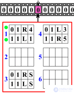
Schematic illustration of the operation of a Turing machine.
The basic idea underlying the Turing machine is very simple. A Turing machine is an abstract machine (automaton) operating on a tape of individual cells in which symbols are recorded. The machine also has a head for writing and reading symbols from the cells, which can move along the tape. At each step, the machine reads the symbol from the cell pointed to by the head, and, based on the symbol read and the internal state, takes the next step. In doing so, the machine may change its state, write a different symbol into the cell, or move the head one cell to the right or left.
Based on the study of these machines, the Turing thesis (the fundamental hypothesis of algorithms) was put forward:
 |
Some algorithm for finding the values of a function defined over a certain alphabet exists if and only if the function is Turing-computable, that is, when it can be computed on a Turing machine. |  |
This thesis is an axiom, a postulate, and cannot be proved by mathematical methods, since an algorithm is not itself a precise mathematical concept.
Recursive functions
Every algorithm can be associated with the function it computes. However, the question arises whether an arbitrary function can be matched with a Turing machine, and if not, for which functions does an algorithm exist? Investigation of these questions led to the creation, in the 1930s, of the theory of recursive functions.
The class of computable functions was formulated in a manner resembling the construction of an axiomatic theory on the basis of a system of axioms. First, the simplest functions were chosen, whose computability is obvious. Then rules (operators) were formulated for constructing new functions from existing ones. The required class of functions consists of all functions that can be obtained from the simplest ones by applying these operators.
Similarly to Turing's thesis, in the theory of computable functions a hypothesis was proposed, known as Church's thesis:
|
A numerical function is algorithmically computable if and only if it is partially recursive. | |
The proof that the class of computable functions coincides with the class of functions computable by Turing takes place in two steps: first it is proved that the simplest functions can be computed on a Turing machine, and then that the functions obtained by applying the operators can also be computed.
Thus, informally, an algorithm can be defined as a precise system of instructions defining a discrete, deterministic process which leads from initial data (the input) to the desired result (the output), if it exists, in a finite number of steps; if the desired result does not exist, the algorithm either never terminates or reaches a dead end.
Markov normal algorithm
A Markov normal algorithm is a system of sequential applications of substitutions that implement specific procedures for obtaining new words from base words built from the symbols of some alphabet. Like the Turing machine, normal algorithms do not carry out the computations themselves: they merely transform words by replacing letters according to given rules[10].
A function that can be realized by a normal algorithm is called normally computable — that is, an algorithm which transforms every word from the set of admissible input data of the function into its initial values[11]..
The creator of the theory of normal algorithms, A. A. Markov, put forward a hypothesis known as Markov's normalization principle:
|
For finding the values of a function defined over a certain alphabet, some algorithm exists if and only if the function is normally computable. | |
Like the theses of Turing and Church, Markov's normalization principle cannot be proved by mathematical means.
However, the formal definition of an algorithm given above may in some cases be too strict. Sometimes there is a need to use random variables[12]. An algorithm whose operation is determined not only by the initial data but also by values obtained from a random number generator is called stochastic (or randomized, from the English "randomized algorithm")[13]. Stochastic algorithms are often more efficient than deterministic ones, and in some cases are the only way to solve a problem[12].
In practice, a pseudorandom number generator is used instead of a true random number generator.
However, stochastic algorithms should be distinguished from methods that give a correct result with high probability. Unlike a method, an algorithm produces correct results even after prolonged operation.
Some researchers allow for the possibility that a stochastic algorithm may give an incorrect result with some known probability. In that case, stochastic algorithms can be divided into two types[14]:
For some problems, the formalizations named above may hinder the search for solutions and the conduct of research. To overcome these obstacles, modifications of the "classical" schemes were developed, as well as new models of algorithms. In particular, one can mention:
and others.
The types of algorithms, as logical-mathematical means, reflect the indicated components of human activity and tendencies, while the algorithms themselves depend on the goal, the initial conditions of the problem, and the ways of solving it. It is worth emphasizing the fundamental difference between computational algorithms, which transform certain input data into output data (it is precisely these that are formalized by the Turing, Post, and RAM machines, Markov normal algorithms, and recursive functions mentioned above), and interactive algorithms (even in Turing's own work one finds the C-machine, from the English "choice," which waits for external influence, in contrast to the classical A-machine, where all initial data are given before the computation begins and the output data are unavailable until the computation ends). The latter are intended for interaction with some control object and are designed to ensure the correct issuance of control actions depending on the evolving situation, as reflected by signals received from the controlled object[15][16]. In some cases a control algorithm does not envisage termination at all (for example, it maintains an infinite loop waiting for events, to which a corresponding response is issued), yet despite this it is considered entirely correct.
One can also distinguish the following types of algorithms:
The numbering of algorithms plays an important role in their study and analysis[18]. Since any algorithm can be specified as a finite word (represented as a finite sequence of symbols of some alphabet), and the set of all finite words in a finite alphabet is countable, the set of all algorithms is also countable. This means there exists a one-to-one correspondence between the set of natural numbers and the set of algorithms, that is, it is possible to assign a number to each algorithm.
The numbering of algorithms is at the same time a numbering of all algorithmically computable functions, and any function may have an infinite number of numbers.
The existence of a numbering allows one to work with algorithms in the same way as with numbers. Numbering is especially useful in the study of algorithms that operate on other algorithms.
Formalizing the concept of an algorithm made it possible to investigate the existence of problems for which no algorithm for finding a solution exists. It was subsequently proved that it is impossible to algorithmically compute solutions to a number of problems, which makes it impossible to solve them on any computing device. A function  is called computable if there exists a Turing machine that computes the value {\displaystyle f} for all elements of the function's domain. If no such machine exists, the function {\displaystyle f} is called uncomputable. A function is considered uncomputable even if there exist Turing machines capable of computing the value for a subset of the entire set of input data[19].
The case in which the result of computing a function is a logical value «true» or «false» (or the set {0, 1}) is called a problem, which may be decidable or undecidable, depending on the computability of the function
It is important to precisely specify the admissible set of input data, since a problem may be decidable for one set and undecidable for another.
One of the first problems for which undecidability was proved is the halting problem. It is formulated as follows:
Given a description of a program for a Turing machine, it is required to determine whether the program will finish running in a finite amount of time or will run forever, given some input data
The proof of the undecidability of the halting problem is important because other problems can be reduced to it. For example, the simple halting problem can be reduced to the halting-on-empty-string problem (where one must determine, for a given Turing machine, whether it will halt when run on an empty string), thereby proving the undecidability of the latter
Along with the spread of information technologies, the risk of software failures has increased. One way of avoiding errors in algorithms and their implementations is to prove the correctness of systems by mathematical means.
The use of mathematical apparatus for analyzing algorithms and their implementations is called formal methods. Formal methods involve the application of formal specifications and, usually, a set of tools for parsing and proving properties of specifications. Abstracting away from implementation details makes it possible to establish properties of a system independently of its implementation. Moreover, the precision and unambiguity of mathematical statements makes it possible to avoid the ambiguity and imprecision of natural languages[21].
According to Richard Mace's hypothesis, «avoiding errors is better than fixing errors»[22]. According to Hoare's hypothesis, «proving programs solves the problem of correctness, documentation, and compatibility»[23]. Proving the correctness of programs makes it possible to identify their properties with respect to the entire range of input data. For this purpose, the concept of correctness has been divided into two types:
When proving correctness, the text of a program is compared with a specification of the desired input-output relationship. For Hoare-style proofs, this specification takes the form of statements called preconditions and postconditions. Together with the program itself, these are also called a Hoare triple. These statements are written
P{Q}R
where P is the precondition, which must hold before running the program Q, and R is the postcondition, which is true after the program finishes running.
Formal methods have been successfully applied to a wide range of problems, in particular: the design of electronic circuits, artificial intelligence, automatic railway systems, microprocessor verification, specification of standards, and the specification and verification of programs[24].
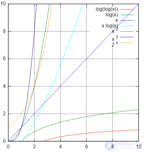
Graphs of the functions given in the table below.
A common criterion for evaluating algorithms is running time and the order of growth of running time as a function of the size of the input data.
For each specific problem, some number is defined, called its size. For example, the size of a matrix multiplication problem could be the largest dimension of the multiplied matrices, while for graph problems the size could be the number of edges in the graph.
The time an algorithm spends as a function of the problem size } is called the time complexity of that algorithm, T(n). The asymptotic behavior of this function as the problem size increases is called asymptotic time complexity, and the «big O» notation is used to denote it. For example, if an algorithm processes input data of size in time cn², where c is some constant, then the time complexity of such an algorithm is said to be O(n²).
Asymptotic complexity is important because it is a characteristic of the algorithm, not of its specific implementation: by «optimizing» operations, without replacing the algorithm, one can change only the multiplicative constant c, but not the asymptotics. As a rule, it is precisely asymptotic complexity that is the main factor determining the size of the problems an algorithm is able to handle.
Often during the development of an algorithm, an attempt is made to reduce the asymptotic time complexity for worst-case scenarios. In practice, however, there are cases where an algorithm that «usually» runs quickly is sufficient.
Roughly speaking, the analysis of average asymptotic time complexity can be divided into two types: analytical and statistical. The analytical method gives more precise results but is difficult to use in practice. On the other hand, the statistical method allows a faster analysis of complex problems[26].
The following table lists common asymptotic complexities with comments[27].
| Complexity | Comment | Examples |
|---|---|---|
| O(1) | Constant running time does not depend on the size of the problem | Expected search time in a hash table |
| O(log log n) | Very slow growth of the required time | Expected running time of interpolation search of n elements |
| O(log n) | Logarithmic growth — doubling the size of the problem increases the running time by a constant amount | Computing xn; Binary search in an array of n elements |
| O(n) | Linear growth — doubling the size of the problem doubles the required time as well | Addition/subtraction of numbers of n digits; Linear search in an array of n elements |
| O(n log n) | Linearithmic growth — doubling the size of the problem increases the required time by a little more than twice | Merge sort or heap sort of n elements; the lower bound of comparison sorting of n elements |
| O(n²) | Quadratic growth — doubling the size of the problem increases the required time fourfold | Elementary sorting algorithms |
| O(n³) | Cubic growth — doubling the size of the problem increases the required time eightfold | Ordinary matrix multiplication |
| O(cn) | Exponential growth — increasing the size of the problem by 1 leads to a c-fold increase in the required time; doubling the size of the problem squares the required time | Some traveling salesman problems, brute-force search algorithms |
An algorithm is a precisely defined instruction, by consistently applying which to input data one can obtain a solution to a problem. For every algorithm there is a certain set of objects admissible as input data. For example, in the algorithm for dividing real numbers, the dividend can be any number, while the divisor cannot equal zero.
An algorithm is normally used to solve not a single specific problem, but a certain class of problems. Thus, the addition algorithm applies to any pair of natural numbers. This expresses its property of generality, that is, the possibility of applying the same algorithm repeatedly to any problem of a given class.
For the development of algorithms and programs, algorithmization is used — the process of systematically composing algorithms to solve applied problems. Algorithmization is considered a mandatory stage in the process of developing programs and solving problems on computers. It is precisely for applied algorithms and programs that determinism, effectiveness and generality, as well as the correctness of the results of solving the stated problems, are fundamentally important.
An algorithm is a clear and precise prescription for an executor to perform a sequence of actions aimed at achieving a goal.
Forms of writing an algorithm:
Usually, at first (at the idea level) an algorithm is described in words, but as it approaches implementation it acquires increasingly formal outlines and a formulation in a language understandable to the executor (for example, machine code).
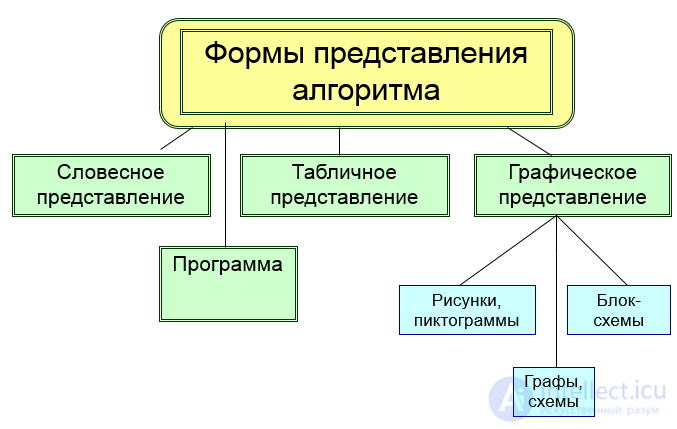
Figure . forms of writing algorithms
A graph is a geometric object consisting of vertices and the arcs connecting the vertices. In the algorithm for analyzing the structure of a sentence, the vertices are the parts of the sentence, the arcs show the connections between parts of the sentence, and the direction of the arcs shows the sequence of the analysis (the order of the algorithm's actions).
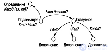
Figure . An example of writing an algorithm in the form of a graph
Standard graphical objects of flowcharts
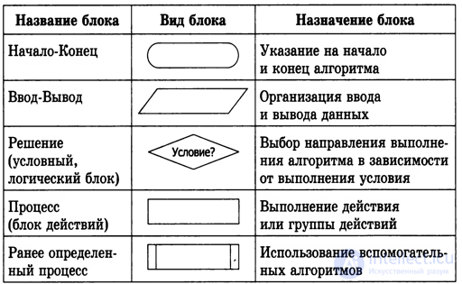
Typical algorithmic structures
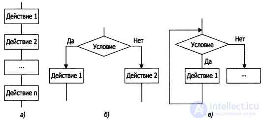
Although the definition of an algorithm only requires the finiteness of the number of steps needed to achieve the result, in practice performing a huge number of steps leads to a long execution of programs, and there are usually other constraints as well (on program size, on permissible actions). In this regard, such notions as the complexity of an algorithm are introduced (time complexity, program-size complexity, computational complexity, and others).
For each problem there may exist a multitude of algorithms leading to the goal. Increasing the efficiency of algorithms has been one of the tasks of computer science since the 1940s, and in this connection a number of algorithms that are more efficient in the asymptotic sense have been built for traditional problems (for example, fast multiplication algorithms[en], the Chudnovsky algorithm for computing the number  ).
).
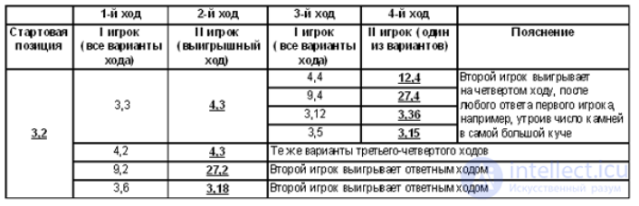
As an illustration — of how they "came to an agreement," not a computational one — let us give an algorithmized description of a conversation between the well-known postman Pechkin and the Talking Starling. The numbering of steps in the verbal description of the algorithm, in the corresponding flowchart (Fig. A1-1) and in the diagram (Fig. A1-2), coincides.
The concept of an algorithm is directly related to the notion of an executor of the algorithm
The relationship between the concepts is shown in the figure:
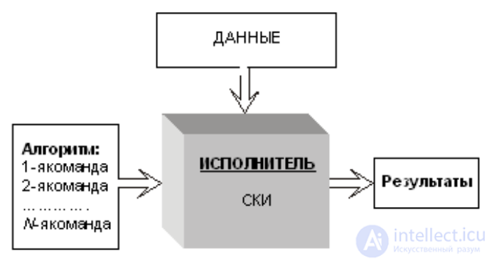

Figure Diagram of the functioning of an algorithm executor
The set of commands that an executor can perform makes up the executor's instruction set (EIS). The algorithm is built from the commands of the EIS. The objects on which the executor can perform actions make up the so-called executor's environment. The data and results shown in the figure are objects belonging to the executor's environment.
The basic properties of an algorithm (discreteness, understandability, definiteness, finiteness) ensure the possibility of the executor's formal work. It follows from this that the executor of algorithms can be an automatic device. The class of problems that an executor is oriented toward solving is determined by its instruction set.
In the methodology of teaching algorithmization, it is customary to distinguish two categories of executors: executors working “in an environment,” and executors working with quantities. For the first category, the executor's environment can be a sheet (screen) on which the executor forms images (drawings, diagrams, etc.); a maze that the executor must overcome; objects that the executor must arrange in a certain order, and so on.
Executors working with quantities are intended for processing numerical or symbolic information. An executor whose instruction set includes arithmetic and logical operations can solve computational problems. Its input data and results are numbers. A universal executor of algorithms for working with quantities is the computer.
The Euclidean algorithm is an efficient method for computing the greatest common divisor (GCD). Named after the Greek mathematician Euclid; one of the oldest algorithms still in use today.
Described in Euclid's «Elements» (approximately 300 years BC), namely in Books VII and X. The seventh book describes the algorithm for integers, while the tenth describes it for the lengths of segments.
There are several variants of the algorithm; below is a recursive version written in pseudocode:
Algorithm 1.
function gcd(a, b)
    if b = 0
       return a
    else
       return gcd(b, a mod b)
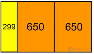
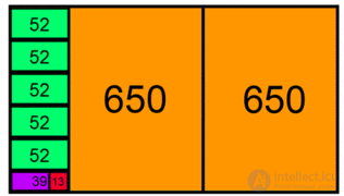
Illustration of the execution of the Euclidean algorithm for computing the GCD of 1599 and 650.
GCD of 1599 and 650:
| Step 1 | 1599 = 650*2 + 299 |
| Step 2 | 650 = 299*2 + 52 |
| Step 3 | 299 = 52*5 + 39 |
| Step 4 | 52 = 39*1 + 13 |
| Step 5 | 39 = 13*3 + 0 |
Algorithm 1. Postman Pechkin and the Jackdaw
Postman Pechkin knocks on the door - "knock-knock".
If the Jackdaw hears the knock, then go to step 3, otherwise - to step 1. {If the bird is a bit deaf or not at home, then Pechkin is not to be envied.}
Jackdaw: "Who's there?"
If Pechkin hears the question "who's there?" {and if the postman himself is hard of hearing, then his affairs are again lamentable}, then go to step 5, otherwise - to step 1.
Pechkin: "It's me, postman Pechkin. Open the door. I've brought a letter for your Boy."
If the Jackdaw opens the door {we hope the heroic bird is up to it, otherwise poor Pechkin is once again in a hopeless situation, since the process will not terminate}, then go to step 7, otherwise - go to step 1.
Postman Pechkin hands over the envelope with the letter.
{The comments in brackets, here and above, are meant to demonstrate, even in such a simple example, how many pitfalls await a programmer debugging a program if the algorithm is not sufficiently
продолжение следует...
Часть 1 Algorithm: Concept, Terminology, Properties, and Notation
Часть 2 See also - Algorithm: Concept, Terminology, Properties, and Notation

Comments