
Lecture
A* (pronounced "A-star") — is a graph traversal and pathfinding algorithm that is used in many areas of computer science due to its completeness, optimality, and optimal efficiency. Given a weighted graph, a source node, and a target node, the algorithm finds the shortest path (with respect to the given weights) from the source to the target.
One of its main practical drawbacks is its space complexity, where d — is the depth of the shallowest solution (the length of the shortest path from the source node to any given target node), and b — is the branching factor (the maximum number of successors for any given state), since it stores all generated nodes in memory. Thus, in practical travel-routing systems it generally loses out to algorithms that can preprocess the graph to achieve better performance, as well as to memory-bounded approaches; however, A* still remains the best solution in many cases.
Peter Hart, Nils Nilsson and Bertram Raphael of the Stanford Research Institute (now SRI International) first published the algorithm in 1968. It can be viewed as an extension of Dijkstra's algorithm. A* achieves better performance by using a heuristic to guide the search.
Compared to Dijkstra's algorithm, the A* algorithm finds only the shortest path from a specified source to a specified target, rather than a tree of shortest paths from the specified source to all possible targets. This is a necessary trade-off for using a heuristic aimed at a specific target. For Dijkstra's algorithm, since the entire tree of shortest paths is generated, every node is a target, and there can be no heuristic aimed at a specific target.
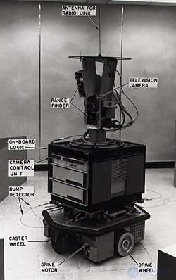
A* was invented by researchers working on path planning for the Shakey the robot.
A* was created as part of the Shakey project, whose goal was to build a mobile robot that could plan its own actions. Nils Nilsson originally proposed using the Graph Traverser algorithm to plan Shakey's path. Graph Traverser is guided by a heuristic function h ( n ), an estimated distance from node n to the goal node: it completely ignores g ( n ), the distance from the start node to n. Bertram Raphael proposed using the sum, g ( n )+ h ( n ). Peter Hart invented the concepts we now call admissibility and consistency of heuristic functions. A* was originally designed for finding least-cost paths, where the cost of a path is the sum of its costs, but it has been shown that A* can be used to find optimal paths for any problem satisfying the conditions of a cost algebra.
The original 1968 A* paper contained a theorem stating that no A*-type algorithm could expand fewer nodes than A*, if the heuristic function is consistent and A*'s conflict-resolution rule is chosen appropriately. A "correction" was published a few years later, claiming that consistency is not required, but this was shown to be false in 1985 in the definitive study of A*'s optimality (now called optimal efficiency) by Dechter and Pearl, which gave an example of an A* variant with a heuristic that was admissible but not consistent, expanding arbitrarily more nodes than an alternative A*-type algorithm.

The A* pathfinding algorithm, moving through a randomly generated maze
Illustration of an A* search for finding a path between two points on a graph. From left to right, an increasingly informative heuristic is used that favors points closer to the goal.
A* is an informed search algorithm, or a "best-first" search, meaning it is formulated in terms of weighted graphs: starting from a given start node of the graph, it seeks to find a path to a given target node with the lowest cost (least distance traveled, shortest time, etc.). It does this by maintaining a tree of paths originating at the start node, and extending those paths one edge at a time until the target node is reached.
At each iteration of its main loop, A* needs to determine which of its paths to extend. It does this based on the cost of the path and an estimate of the cost required to extend the path to the goal. Specifically, A* selects the path that minimizes

where n — is the next node on the path, g ( n ) — is the cost of the path from the start node to n, and h ( n ) — is a heuristic function that estimates the cost of the cheapest path from n to the goal. The heuristic function is problem-specific. If the heuristic function is admissible — that is, it never overestimates the actual cost of reaching the goal — A* is guaranteed to return a least-cost path from start to goal.
Typical implementations of A* use a priority queue to repeatedly select the node with the minimum (estimated) cost to expand. This priority queue is known as the open set, fringe, or frontier. At each step of the algorithm, the node with the lowest f ( x ) value is removed from the queue, the f and g values of its neighbors are updated accordingly, and these neighbors are added to the queue. The algorithm continues until a removed node (thus the node with the lowest f value among all nodes in the frontier) is the target node. The f value of that target is then also the cost of the shortest path, since h at the goal is zero for an admissible heuristic.
The algorithm described so far only produces the length of the shortest path. To find the actual sequence of steps, the algorithm can easily be revised so that each node on the path keeps track of its predecessor. After running this algorithm, the end node will point to its predecessor, and so on, until the predecessor of some node is the start node.
For example, when finding the shortest route on a map, h ( x ) might represent the straight-line distance to the goal, since that is physically the smallest possible distance between any two points. For a grid map from a video game, using Taxicab distance or Chebyshev distance becomes a better choice depending on the set of available moves (4 or 8 directions).
If the heuristic h satisfies the additional condition h ( x ) ≤ d ( x , y ) + h ( y ) for every edge ( x , y ) of the graph (where d denotes the length of that edge), then h is called monotonic or consistent. With a consistent heuristic, A* is guaranteed to find an optimal path without processing any node more than once, and A* is equivalent to running Dijkstra's algorithm with the reduced cost d' ( x , y ) = d ( x , y ) + h ( y ) − h ( x ).
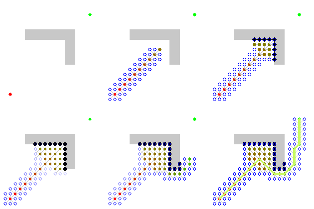
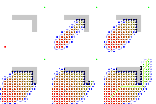 Illustration of an A* search for finding a path from a start node to an end node in a robot motion-planning problem. The empty circles represent nodes in the open set, i.e. those still to be explored, while the filled circles are in the closed set. The color of each closed node indicates its distance from the goal: the greener, the closer. At first you can see A* moving in a straight line toward the goal, then, upon encountering an obstacle, it explores alternative routes through the nodes in the open set.
An example of the A* algorithm in action, where the nodes are cities connected by roads, and h(x) — is the straight-line distance to the target point:
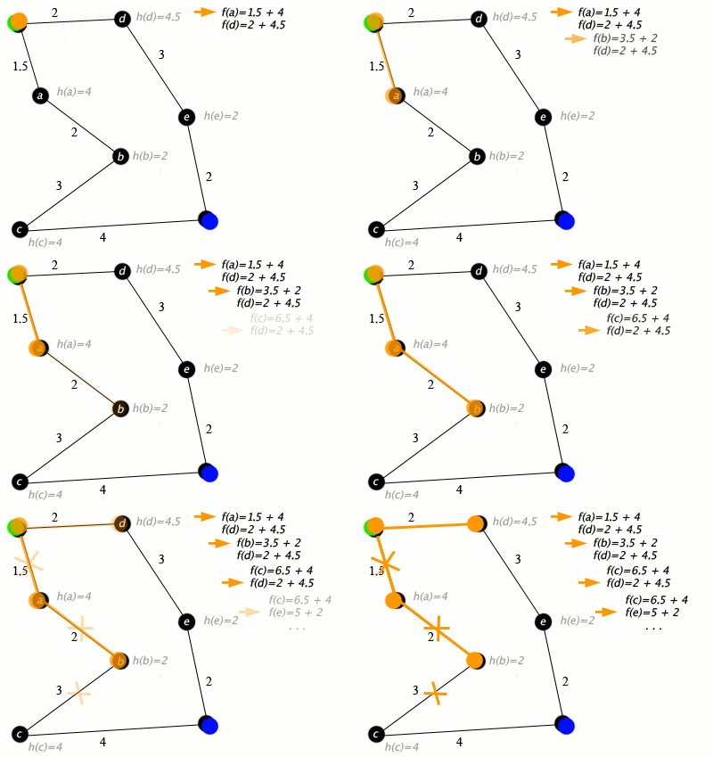
Notation: green: start; blue: goal; orange: visited
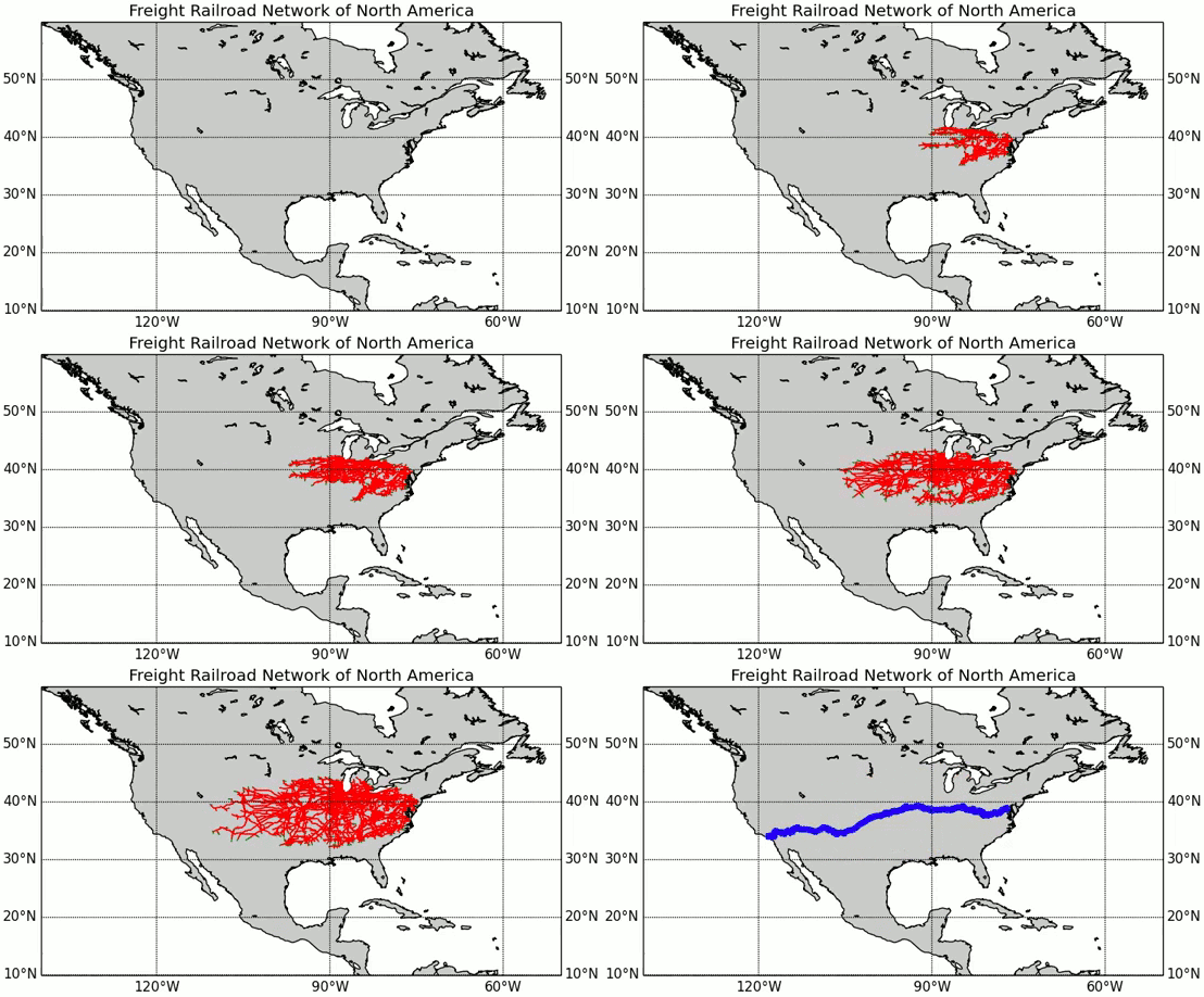
The A* algorithm has real applications. In this example, the edges — are railroads, and h(x) — is the great-circle distance (the shortest possible distance on a sphere) to the goal. The algorithm searches for a path between Washington, D.C., and Los Angeles.
There are a number of simple optimizations or implementation details that can significantly affect the performance of an A* implementation. The first detail worth noting is that the way the priority queue handles ties can significantly affect performance in some situations. If ties are broken and the queue behaves in a LIFO manner, A* will behave like a depth-first search among paths of equal cost (avoiding exploration of more than one equally optimal solution).
When a path is required at the end of the search, a reference to the parent of each node is usually stored. At the end of the search, these references can be used to reconstruct the optimal path. If these references are stored, it can be important that the same node not appear in the priority queue more than once (each entry corresponds to a different path to the node, and each has its own cost). The standard approach here is to check whether the node to be added already appears in the priority queue. If it does, the priority and parent pointers are changed to correspond to the lower-cost path. A standard priority-based binary heap does not directly support the operation of searching for one of its elements, but it can be supplemented with a hash table that maps elements to their position in the heap, allowing this decrease-priority operation to be performed in logarithmic time. Alternatively, a Fibonacci heap can perform the same decrease-priority operations in constant amortized time.
Dijkstra's algorithm, as another example of a uniform-cost search algorithm, can be viewed as a special case of A*, where  for all x.] General depth-first search can be implemented using A* if we consider that there is a global counter C, initialized to a very large value. Each time we process a node, we assign C to all its newly discovered neighbors. After each assignment, we decrement the counter C by one. Thus, the earlier a node is discovered, the higher its
  value. Both Dijkstra's algorithm and depth-first search can be implemented more efficiently without including the value at each node.
On finite graphs with non-negative edge weights, A* is guaranteed to terminate and is complete, i.e. it will always find a solution (a path from start to goal) if one exists. On infinite graphs with a finite branching factor and edge costs that are bounded away from zero  for some fixedε
 ), A* is guaranteed to terminate only if a solution exists.
A search algorithm is considered admissible if it is guaranteed to return an optimal solution. If the heuristic function used by A* is admissible, then A* is admissible. An intuitive «proof» of this is as follows:
Let us call a node closed if it has been visited and is not in the open set. We close a node when we remove it from the open set. The key property of the A* algorithm, whose proof we sketch below, is that when n is closed,
  — is an optimistic estimate (lower bound) of the true distance from start to goal. Therefore, when the goal node, g
 , is closed,
  is no greater than the true distance. On the other hand, it is no less than the true distance, since it is the length of the path to the goal plus the heuristic term.
Now we will see that whenever a node n is closed, — is an optimistic estimate. It suffices to see that whenever the open set is not empty, it has at least one node n on the optimal path to the goal, for which  — is the true distance from the start, since in that case +
  underestimates the distance to the goal, and hence so does the smaller value chosen for the closed vertex. Let
  — be the optimal path from start to goal. Let
  be the last closed node on for which
  — is the true distance from the start to the goal (the start is one such vertex). The next node in has the correct value, since it was updated when was closed, and it is open, since it is not closed.
Algorithm A is optimally efficient with respect to a set of alternative algorithms Alts on a set of problems P if, for every problem P in P and every algorithm A′ in Alts, the set of nodes expanded by A when solving P is a subset (possibly equal) of the set of nodes expanded by A′ when solving P. The definitive study of the optimal efficiency of A* belongs to Rina Dechter and Judea Pearl.[ They considered many definitions of Alts and P in combination with a heuristic for A* that is either simply admissible or is both consistent and admissible. The most interesting positive result they proved is that A* with a consistent heuristic is optimally efficient with respect to all admissible A*-type search algorithms on all «non-pathological» search problems. Roughly speaking, their notion of a non-pathological problem is what we now mean by «before conflict resolution». This result does not hold if the A* heuristic is admissible but not consistent. In this case, Dechter and Pearl showed that there exist admissible A*-type algorithms that can expand arbitrarily fewer nodes than A* on some non-pathological problems.
Optimal efficiency concerns the set of expanded nodes, not the number of node expansions (the number of iterations of A*'s main loop). When the heuristic used is admissible but not consistent, it is possible for a node to be expanded by A* many times, an exponential number of times in the worst case. Under such circumstances, Dijkstra's algorithm can outperform A* by a wide margin. However, later research has shown that this pathological case arises only in certain contrived situations, where the search graph's edge weight is exponential in the size of the graph, and that certain inconsistent (but admissible) heuristics can lead to a reduction in the number of node expansions in an A* search.
A* search that uses a heuristic 5.0(=ε) times larger than a consistent heuristic, and obtains a non-optimal path
Although the admissibility criterion guarantees an optimal solution path, it also means that A* must check all equally worthy paths in order to find the optimal path. To compute approximate shortest paths, the search can be sped up at the expense of optimality by relaxing the admissibility criterion. Often we want to bound this relaxation so as to guarantee that the solution path is no worse than (1 + ε) times the optimal solution path. This new guarantee is called ε-admissible.
There are a number of ε-admissible algorithms:
 -optimal paths overall.
 .
.
 .
.
-optimal.


 , where 0 otherwise
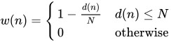 , and where
  is the search depth, and N is the estimated length of the solution path.
 . uses two heuristic functions. The first is the FOCAL list, which is used to select candidate nodes, and the second h F is used to select the most promising node from the FOCAL list.
 , where A and B are constants. If no node can be selected, the algorithm falls back to the function
  , where C and D are constants.
 , where
 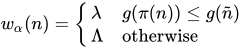 , where λ and Λ are constants
  , π( n ) is the parent node of n, and ñ is the most recently expanded node.
As a heuristic search algorithm, A*'s performance largely depends on the quality of the heuristic function. . If the heuristic closely approximates the true cost to the goal, A* can significantly reduce the number of node expansions. On the other hand, a poor heuristic can lead to many unnecessary expansions.
In the worst case, A* expands all nodes for which
  , where
 is the cost of the optimal goal node.
Suppose there is a node in the open list
  , and it is the next node to be expanded. Since the goal node has
 , , the goal node will have a smaller f value and will be expanded before .
Therefore A* never expands nodes with .
.
Suppose there is an optimal algorithm that expands fewer nodes, in the worst case using the same heuristic. This means there must be some node such that  , yet the algorithm chooses not to expand it.
Now consider a modified graph, where a new edge of cost (
( ) is added fromto the goal. If
  , then the new optimal path passes through. However, since the algorithm still avoids expanding, it will miss the new optimal path, violating its optimality.
Therefore, no optimal algorithm including A* can expand fewer nodes thanin the worst case.
The worst-case complexity of A* is often described as , whereb
 is the branching factor and
  is the depth of the shallowest goal. While this gives a rough intuition, it does not accurately reflect the actual behavior of A*.
A more accurate estimate takes into account the number of nodes  . Ifεis the smallest possible difference in
  -cost between individual nodes, then A* can expand up to:

In the worst case this reflects both time and space complexity.
The space complexity of A* is roughly the same as that of all other graph search algorithms, since it stores all generated nodes in memory. In practice, this turns out to be the biggest drawback of A* search, which has led to the development of memory-bounded heuristic searches such as iterative-deepening A*, memory-bounded A*, and SMA*.
A* is often used to solve the general path-finding problem in applications such as video games, but it was originally developed as a general graph traversal algorithm. It is applied in various tasks, including the parsing problem using stochastic grammars in natural language processing. Other applications include information retrieval with online learning.
The difference between A* and the greedy best-first search algorithm is that A* takes into account the cost/distance traveled g ( n ) .
Some common variants of Dijkstra's algorithm can be regarded as a special case of A*, where the heuristic  for all nodes; in turn, both Dijkstra's algorithm and A* are special cases of dynamic programming. A* itself is a special case of the generalization of branch and bound.
A* is similar to beam search, except that beam search maintains a limit on the number of paths it needs to explore.
A* can also be adapted to a bidirectional search algorithm, but special attention must be paid to the stopping criterion.

Comments