
Lecture
Это окончание невероятной информации про сложность алгоритмов.
...
functions. The original call to mergeSort spawns two new calls for arrays of size n / 2 each. In turn, each of them spawns two more calls with arrays of n / 4 elements, and so on until we get an array of size 1. This diagram is called a recursion tree, because it illustrates the workings of recursion and looks like a tree (more precisely, like an inverted tree with the root at the top and the leaves at the bottom).
Notice that the number of elements in each row remains equal to n. Also note that each calling node uses the results obtained from the nodes it calls for the merge operation. For example, the red node sorts n / 2 elements. To do this, it splits the n / 2 array into two of n / 4 each, recursively calls mergeSort on each of them (the green nodes), and combines the results into a single whole of size n / 2.
As a result, the complexity of each row is Θ( n ). We know that the number of such rows, called the depth of the recursion tree, will be log( n ). The reasoning behind this is the same as we used for binary search. So, we have log( n ) rows with complexity Θ( n ), hence the total complexity of mergeSort is: Θ( n * log( n ) ). This is much better than Θ( n2 ), which selection sort gives us (remember, log( n ) is much smaller than n, so n * log( n ) is also much smaller than n * n = n2).
As you saw in the last example, complexity analysis allows us to compare algorithms in order to understand which of them is better. Based on these considerations, we can now be confident that for large arrays, merge sort will significantly outperform selection sort. Such a conclusion would be difficult to reach if we did not have a theoretical basis for analyzing the algorithms we develop. Undoubtedly, sorting algorithms with running time Θ( n * log( n ) ) are widely used in practice. For example, the Linux kernel uses an algorithm called «heap sort», which has the same running time as merge sort. Note that we will not prove the optimality of these sorting algorithms. This would require far more cumbersome mathematical arguments, but rest assured: from a complexity standpoint, one cannot find a better option.
After studying this article, the intuition you have gained about algorithm complexity analysis should help you create fast programs and focus your optimization efforts on the things that truly have a major impact on execution speed. Together, this will let you work more productively. Moreover, the mathematical language and notations (for example, «Big O») covered in this article will be useful to you when communicating with other software developers about algorithm running times, and, hopefully, you will be able to apply the knowledge gained in practice.
There are several ways to measure the complexity of an algorithm. Programmers usually focus their attention on the speed of an algorithm, but other indicators are no less important – requirements for memory volume, free disk space. Using a fast algorithm will not produce the expected results if running it requires more memory than the computer has.
When comparing different algorithms, it is important to know how their complexity depends on the volume of input data. Suppose that, with one sorting method, processing a thousand numbers takes 1 second, and processing a million numbers takes 10 seconds, while using another algorithm might require 2 seconds and 5 seconds respectively. Under such conditions, it is impossible to say unambiguously which algorithm is better.
In general, the complexity of an algorithm can be estimated by order of magnitude. An algorithm has complexity O(f(n)) if, as the size N of the input data increases, the execution time of the algorithm grows at the same rate as the function f(N). Let us consider code that, for a matrix A[NxN], finds the maximum element in each row.
for i:=1 to N do

begin

max:=A[i,1];

for j:=1 to N do

begin

if A[i,j]>max then

max:=A[i,j]

end;

writeln(max);

end;
In this algorithm, the variable i changes from 1 to N. With each change of i, the variable j also changes from 1 to N. During each of the N iterations of the outer loop, the inner loop also runs N times. The total number of iterations of the inner loop equals N*N. This defines the algorithm's complexity as O(N^2).
When estimating the order of complexity of an algorithm, only the part that grows the fastest should be used. Suppose that the running cycle is described by the expression N^3+N. In that case, its complexity will equal O(N^3). Considering the fastest-growing part of the function makes it possible to estimate the behavior of the algorithm as N increases. For example, at N=100, the difference between N^3+N=1000100 and N=1000000 is only 100, which amounts to 0.01%.
When calculating O, constant factors in expressions may be disregarded. An algorithm with a running step of 3N^3 is considered as O(N^3). This makes the dependence of the O(N) relationship on the change in the size of the problem more apparent.
The most complex parts of a program are usually the execution of loops and the calling of procedures. In the previous example, the entire algorithm was carried out using two loops.
If one procedure calls another, then the complexity of the latter must be assessed more carefully. If it executes a fixed number of instructions (for example, printing output), this practically has no effect on the complexity estimate. But if the called procedure executes O(N) steps, the function can significantly increase the complexity of the algorithm. And if the procedure is called inside a loop, the effect can be much greater.
As an example, let us consider two procedures: Slow with complexity O(N^3) and Fast with complexity O(N^2).
procedure Slow;

var

i,j,k: integer;

begin

for i:=1 to N do

for j:=1 to N do

for k:=1 to N do

{some action}

end;

procedure Fast;

var

i,j: integer;

begin

for i:=1 to N do

for j:=1 to N do

Slow;

end;

procedure Both;

begin

Fast;

end;
If, in the inner loops of procedure Fast, procedure Slow is called, then the complexities of the procedures are multiplied. In this case, the complexity of the algorithm is O(N^2 )*O(N^3 )=O(N^5).
But if the main program calls the procedures one after another, their complexities are added: O(N^2 )+O(N^3 )=O(N^3). The following fragment has exactly this complexity:
procedure Slow;

var

i,j,k: integer;

begin

for i:=1 to N do

for j:=1 to N do

for k:=1 to N do

{some action}

end;

procedure Fast;

var

i,j: integer;

begin

for i:=1 to N do

for j:=1 to N do

{some action}

end;

procedure Both;

begin

Fast;

Slow;

end;
function Factorial(n: Word): integer;

begin

if n > 1 then

Factorial:=n*Factorial(n-1)

else

Factorial:=1;

end;procedure DoubleRecursive(N: integer);
begin
if N>0 then
begin
DoubleRecursive(N-1);
DoubleRecursive(N-1);
end;
end;
An estimate of an algorithm's complexity up to order is an upper bound on the algorithm's complexity. If a program has a large order of complexity, this does not at all mean that the algorithm will actually run for a long time. On certain data sets, the execution of an algorithm takes far less time than one might expect based on its complexity. For example, let us consider code that searches for a given element in the vector A.
function Locate(data: integer): integer;

var

i: integer;

fl: boolean;

begin

fl:=false; i:=1;

while (not fl) and (i<=N) do

begin

if A[i]=data then

fl:=true

else

i:=i+1;

end;

if not fl then

i:=0;

Locate:=I;

end;
If the sought element is at the end of the list, the program will have to execute N steps. In that case, the algorithm's complexity will be O(N). In this worst case, the algorithm's running time will be at its maximum.
On the other hand, the sought element may be located at the first position in the list. The algorithm will only have to take one step. This case is called the best case, and its complexity can be estimated as O(1).
Both of these cases are unlikely. What interests us most is the expected case. If the elements of the list are initially arranged in random order, the sought element could turn out to be anywhere in the list. On average, N/2 comparisons will be required to find the desired element. This means that the average complexity of this algorithm is O(N/2)=O(N).
In this case, the average and expected complexity coincide, but for many algorithms the worst case differs greatly from the expected one. For example, quicksort has a worst-case complexity of order O(N^2), while its expected behavior is described by the estimate O(N*log(N)), which is much faster.
The complexity of algorithms is usually assessed by execution time or memory used. In both cases, complexity depends on the size of the input data: an array of 100 elements will be processed faster than a similar one of 1000. At the same time, hardly anyone is interested in the exact time: it depends on the processor, the data type, the programming language, and many other parameters. Only the asymptotic complexity matters, i.e., the complexity as the size of the input data tends to infinity.
Suppose some algorithm needs to perform 8n3 + 7n conditional operations to process n elements of input data. As n increases, the total running time will be affected much more significantly by raising n to the cube than by multiplying it by 8 or adding 7n. In this case, the time complexity of this algorithm is said to be O(n3), i.e., it depends on the size of the input data cubically.
The use of the capital letter O (or the so-called O-notation) comes from mathematics, where it is used to compare the asymptotic behavior of functions. Formally, O(f(n)) means that the running time of the algorithm (or the amount of memory occupied) grows, depending on the volume of input data, no faster than some constant multiplied by f(n).
This complexity is possessed, for example, by the algorithm for finding the largest element in an unsorted array. We will have to go through all n elements of the array to figure out which one is the maximum.
The simplest example — binary search. If the array is sorted, we can check whether it contains some specific value by the method of halving. We check the middle element; if it is greater than the one we're looking for, we discard the second half of the array — it's certainly not there. If it's smaller, then, conversely, we discard the initial half. And so we continue halving, ultimately checking log n elements.
This complexity is possessed, for example, by the insertion sort algorithm. In its canonical implementation, it consists of two nested loops: one to go through the entire array, and the second to find a place for the next element within the already sorted part. Thus, the number of operations will depend on the size of the array as n * n, i.e., n2.
There are other complexity estimates, but they are all based on the same principle.
It also happens that the running time of an algorithm does not depend on the size of the input data at all. In that case, the complexity is denoted as O(1). For example, to determine the value of the third element of an array, there is no need to either remember the elements or go through them any number of times. It's always enough to simply wait for the third element in the input data stream, and that will be the result, whose computation takes the same amount of time regardless of the amount of data.
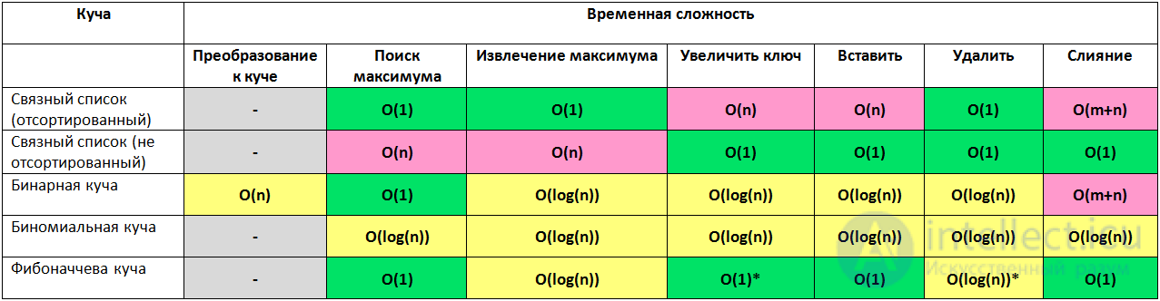
Memory is estimated similarly, when this matters. However, some algorithms may use significantly more memory as the size of the input data increases than others, but run faster in return. And vice versa. This helps in choosing optimal ways of solving problems based on current conditions and requirements.
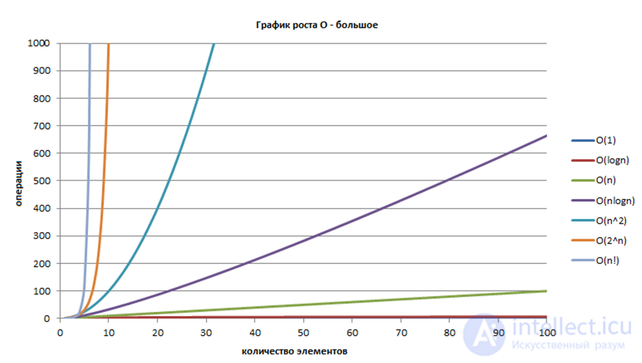
Execution time of an algorithm with a given complexity depending on the size of the input data at a speed of 106 operations per second:
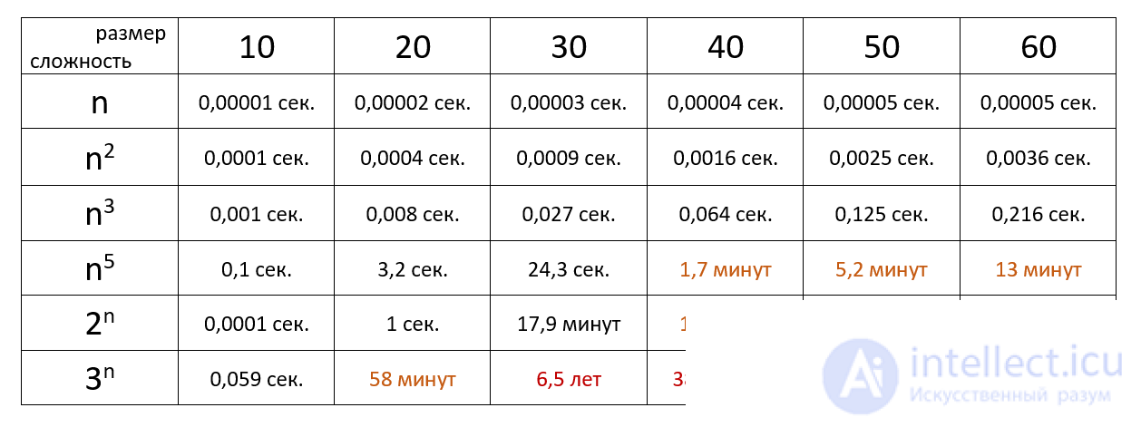
Thus, by running the algorithm with different sets and volumes of data, one can asymptotically plot graphs and determine big O or little o



«Big O notation is a mathematical notation that describes the limiting behavior of a function when the argument tends to a particular value or infinity. It is a member of a family of notations invented by Paul Bachmann, Edmund Landau and others, which are collectively called Bachmann–Landau notations or asymptotic notations».
Put simply, Big O notation describes the complexity of your code using algebraic terms.
To understand what Big O is, we can look at a typical example, O (n²), which is usually pronounced «Big O squared». The letter «n» here represents the size of the input data, and the function «g (n) = n²» inside «O ()» gives us an idea of how complex the algorithm is relative to the amount of input data.
A typical algorithm with complexity O(n²) would be selection sort. Selection sort is a sorting algorithm that iterates over the list to ensure that each element with index i is the i-th smallest/largest element of the list. A visual example.
https://www.youtube.com/embed/Ns4TPTC8whwThe algorithm can be described by the following code. To ensure that the i-th element is the i-th smallest element in the list, this algorithm first scans the list using a for loop. Then, for each element, it uses another for loop to find the smallest element in the rest of the list.
In this scenario we consider the variable List as the input data, so the input size n is the number of elements inside List. Assume that the if statement, and the value assignment bounded by the if statement, take constant time. Then we can find Big O for the SelectionSort function by analyzing how many times the statements are executed.
First, the inner for loop executes the statements inside n times. Then, after incrementing i, the inner for loop executes n-1 times … until it runs one more time, at which point both for loops reach their termination conditions.
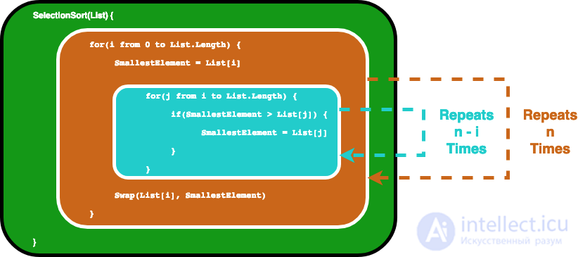
Selection Sort Loops Illustrated
In fact this ultimately gives us a geometric sum, and thanks to middle-school mathematics we find that the inner loop will repeat 1 + 2… + n times, which equals n(n-1)/2 times. If we multiply this out, we get n²/2-n/2.
When we compute Big O, we only care about the dominant terms, and we do not care about the coefficients. Thus, we choose n² as the Big O. We write it as O(n²), and pronounce it as «Big O squared».
Now you may be wondering what these «dominant terms» are? And why don't we care about the coefficients? Don't worry, we will address these questions one by one below.
Once upon a time there lived an Indian king who wanted to reward a sage. The sage asked, as a reward, only for wheat that would fill an entire chessboard.
But under a certain condition: the first cell should have 1 grain of wheat, then 2 grains on the second cell, then 4 on the next … and so on, each cell on the chessboard should have twice as many grains as the previous one. The naive king agreed without hesitation, thinking this was too simple a condition…
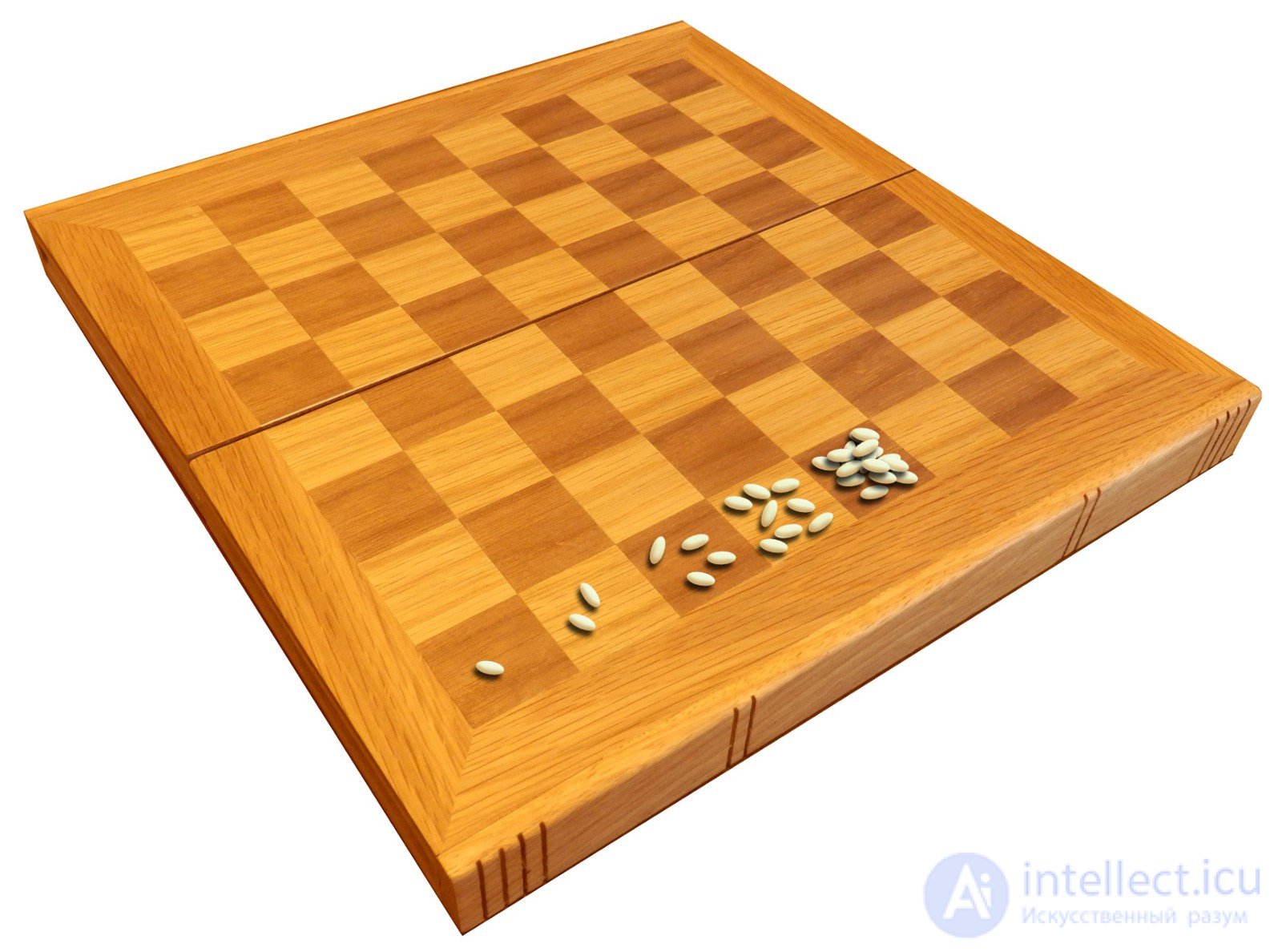
Wheat and Chess Board, Image from Wikipedia
So how much wheat did the king owe the sage? We know that a chessboard has 8 squares by 8 squares, which adds up to 64 squares, so the final square should have 2⁶⁴ grains of wheat. If you do the calculation yourself, you get 1.8446744 * 10¹⁹, that is, about 18 followed by 18 zeros. Assuming each grain of wheat weighs 0.01 grams, this gives us 184,467,440,737 tons of wheat. And 184 billion tons is a lot, isn't it?
Numbers can grow quite fast, can't they? The same logic applies to computer algorithms. If the effort required to perform a task grows exponentially with respect to the size of the input data, the algorithm may eventually become extremely costly.
If you keep doubling 2⁶⁴, the result will quickly be lost beyond significant digits. That is why, when we look at growth rates, we only care about the dominant terms. And since we want to analyze growth with respect to the size of the input, coefficients that merely multiply the number and do not grow with the size of the input carry no useful information.
Below is the formal definition of Big O:
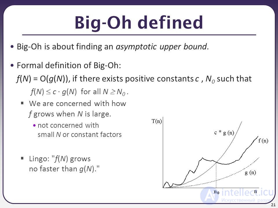
CSE 373 Slides from University of Washington
The formal definition is useful when you need to carry out a mathematical proof. For example, the complexity of selection sort can be defined by the function f (n) = n²/2-n/2, as we discussed in the previous section.
If we let our function g(n) be n², we can find a constant c = 1 and N₀ = 0, provided that N > N₀, where N² will always be greater than N²/2-N/2. We can easily prove this by subtracting N²/2 from both functions, then we can see that N²/2 > -N/2 will be true when N>0. Therefore we can conclude that f(n) = O (n²), in other selection order this is "Big O squared."
You may have noticed a small trick. That is, if you make g(n) grow faster than anything else, O(g(n)) will always be large enough. For example, for any polynomial function you will always be correct in saying that it is O(2ⁿ), because 2ⁿ will eventually always be greater than any polynomial.
Mathematically you would be correct, but usually, when we talk about Big O, we need to know the tight bound (tight bound) of the function. You will learn more about this in the next section.
But before we go further, let's test your understanding with the following question. The answer will be given in the next section.
Question: Suppose an image is represented by a two-dimensional array of pixels. You use a nested for loop to iterate over every pixel (that is, you have a for loop going through all columns, and another loop inside it to go through all rows). What would be the complexity of the algorithm in this case?
Below are the formal mathematical definitions of these notations:
Big O: "f(n) is O(g (n))" if and only if there exist constants c and N₀ such that f(N) ≤ cg(N) for all N> N₀
Little O: "f(n) is o (g(n))", if f(n) is O(g(n)) and f(n) is not Θ(g(n))
Omega: "f(n) is Ω(g(n))" if and only if there exist constants c and N₀ such that f(N) ≥ cg(N) for all N> N₀
Theta: "f (n) is Θ(g (n))" if and only if f(n) is O(g(n)), and f(n) is Ω(g(n))
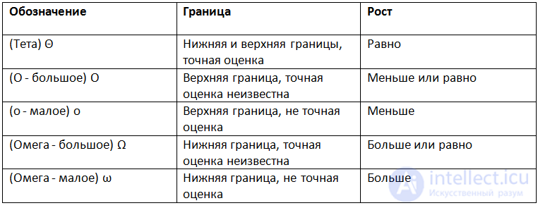
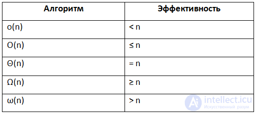
In simple terms:
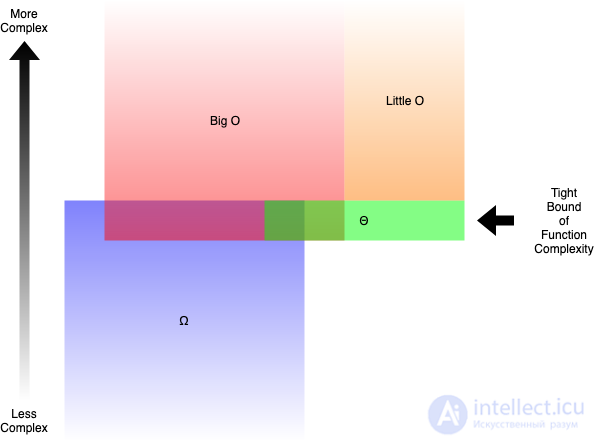
Relationships between Big O, Little O, Omega & Theta Illustrated
For example, the function g(n) = n² + 3n is O(n³), o(n⁴), Θ(n²), and Ω (n). But you would still be correct if you said it is Ω(n²) or O(n²).
In general, when we talk about Big O, we actually mean Theta (Θ Theta). It makes no sense to define an upper bound that far exceeds the scope of the analysis. It would be like solving inequalities by putting ∞ on the larger side, which would almost always formally make you correct.
But how do you determine which functions are more complex than others?
When we try to determine Big O for a specific function g(n), we only care about the dominant term of the function. The dominant term is the term that grows the fastest.
For example, n² grows faster than n, so if we have something like g(n) = n² + 5n + 6, then the Big O will be (n²). If you have ever done some calculus, this is very similar to canceling limits for fractional polynomials, where you only care about the dominant term for the numerators and denominators in the end.
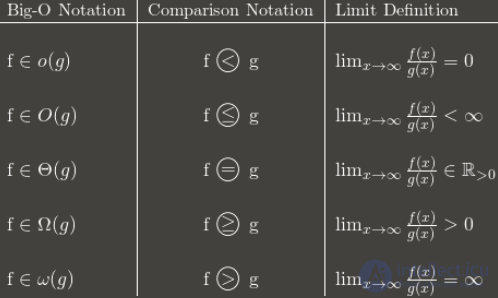
Another way to look at Big O, Image from Stack Overflow
But which function grows faster than others? There are actually quite a few rules.
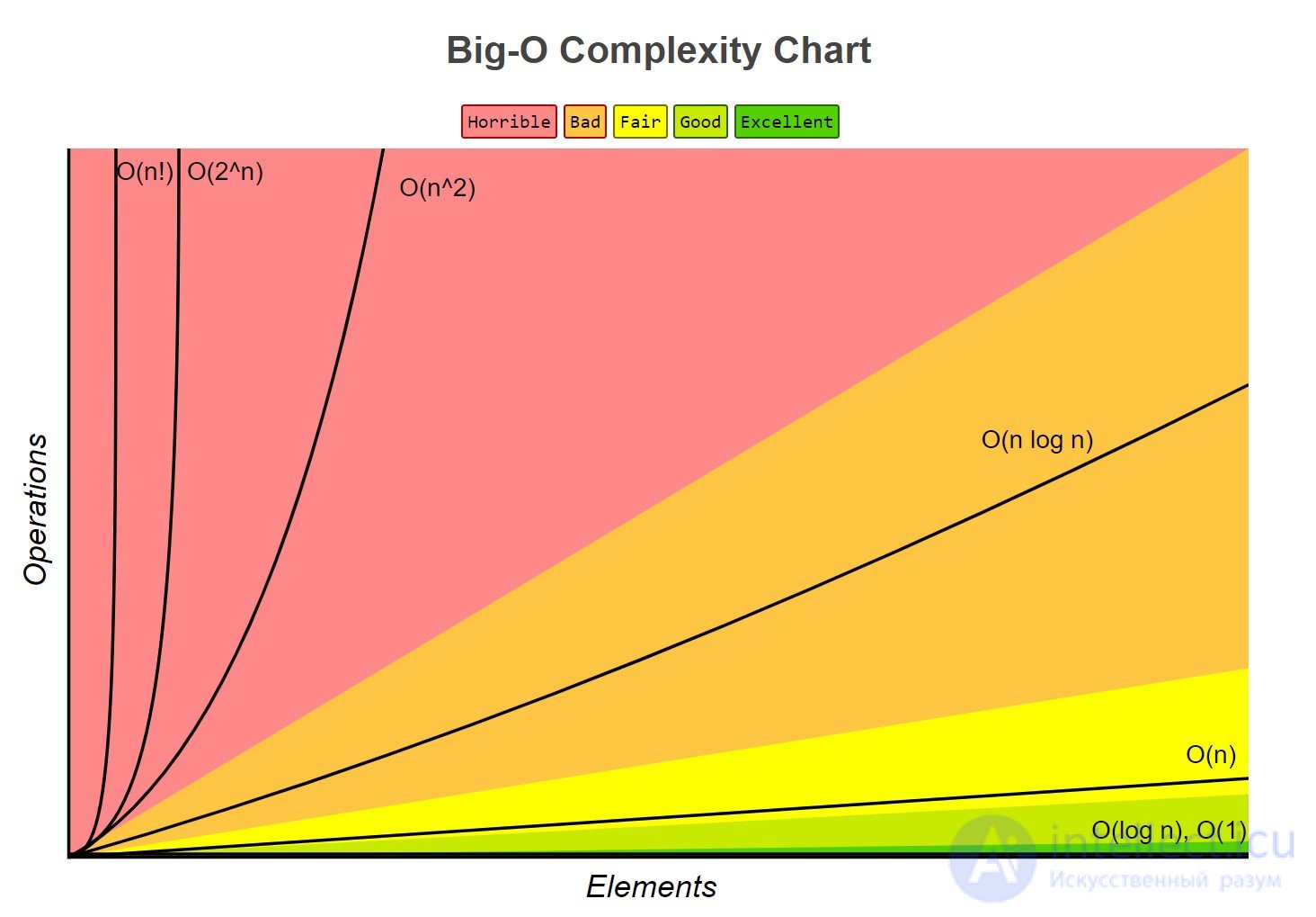
Complexity Growth Illustration from Big O Cheatsheet
Often called "constant time", if you can create an algorithm to solve a problem with O(1), then that would be the best choice of algorithm. In some scenarios, complexity may go below O(1), and then we can analyze it by finding its counterpart O(1/g(n)). For example, O(1/n) is more complex than O(1/n²).
Since complexity is often associated with "divide and conquer" algorithms, O (log(n)) is generally a good complexity to achieve for sorting algorithms. O (log(n)) is less complex than O (√n), because the square root function can be considered a polynomial where the exponent equals 0.5.
For example, O (n⁵) is more complex than O (n⁴).
O (2ⁿ) is more complex than O (n⁹⁹), but O (2ⁿ) is actually less complex than O(1). We usually take 2 as the base for powers and logarithms because in computer science everything tends to be binary, but the base can be changed by changing the coefficients. Unless otherwise specified, the base for logarithms is taken to be 2.
If you are interested in the proofs, look at the Gamma function (Gamma function), which is the analytic continuation of the factorial. The short proof is that both factorials and exponentiation have the same number of multiplications, but the numbers being multiplied grow for factorials while remaining unchanged for exponentiation.
When multiplying, the complexity will be greater than the original, but not greater than the equivalent of multiplying something more complex. For example, O (n*log (n)) is more complex than O (n), but less complex than O (n²), because O (n²) = O (n * n), and n is more complex than log (n). ).
If you'd like, you can test your understanding. Try to rank the following functions from most complex to least. Solutions with detailed explanations can be found in the next section. Some of them are complex enough and may require a deeper understanding of mathematics. When you get to the solution, you will learn more about it.
Question: Arrange the following functions from most complex to least.
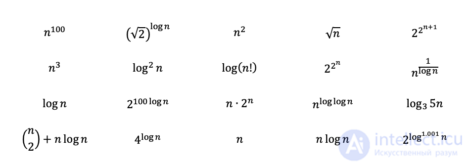
Examples taken from Textbook Problems
Solution to the Question from Section 2:
This was actually a trick question, designed to test your understanding. You might have guessed the answer is O (n²), because there is a nested for loop. But you need to understand that the input is an array of images, and each pixel in the algorithm is visited only once, so the answer is actuallyO (n). In the next section, we will look at other examples similar to this one.
So far, we have only discussed the time complexity of algorithms. That is, we only care about how much time a program will need to complete a task. Also important is the space occupied by a program in memory to perform a task. Space complexity is concerned with how much memory a program will use, and is therefore also an important factor to analyze.
Space complexity works similarly to time complexity. For example, selection sort has a space complexity of O(1), because it stores only a single minimum value and its index for comparison, and the maximum space used does not increase with the size of the input.
Some algorithms, such as bucket sort, have a space complexity of O (n), but this makes it possible to reduce the time complexity to O (1). Bucket sort is a type of sort in which the elements being sorted are distributed among a finite number of separate blocks (buckets, bins), so that all elements in each successive block are always greater than (or less than) those in the previous one. Each block is then sorted separately, either recursively using the same method or a different one. The elements are then placed back into the array.
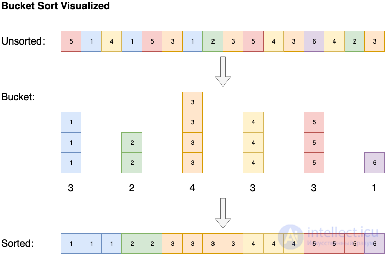
Bucket Sort Visualization
Complexity can also be analyzed as the best case, worst case, average case, and expected case.
As an example, let's look at insertion sort (insertion sort). Insertion sort iterates over all the elements in a list. If an element is greater than its previous element, it inserts the element back until it becomes greater than the previous element.
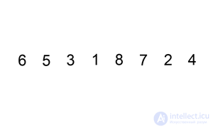
Insertion Sort Illustrated, Image from Wikipedia
If the array is already sorted, no swaps will be performed at all. The algorithm will simply iterate through the array once, resulting in a time complexity of O (n). Therefore, we would say that the best-case time complexity of insertion sort is O (n). A complexity of O (n) is also often called linear complexity.
Sometimes an algorithm can simply be unlucky. For example, quicksort will have to go through the list in O (n) if the elements are sorted in reverse order, but on average this algorithm sorts the array in O (n * log(n)). As a rule, when we estimate the time complexity of an algorithm, we look at its worst-case performance. We will talk more about this and about quicksort in the next section.
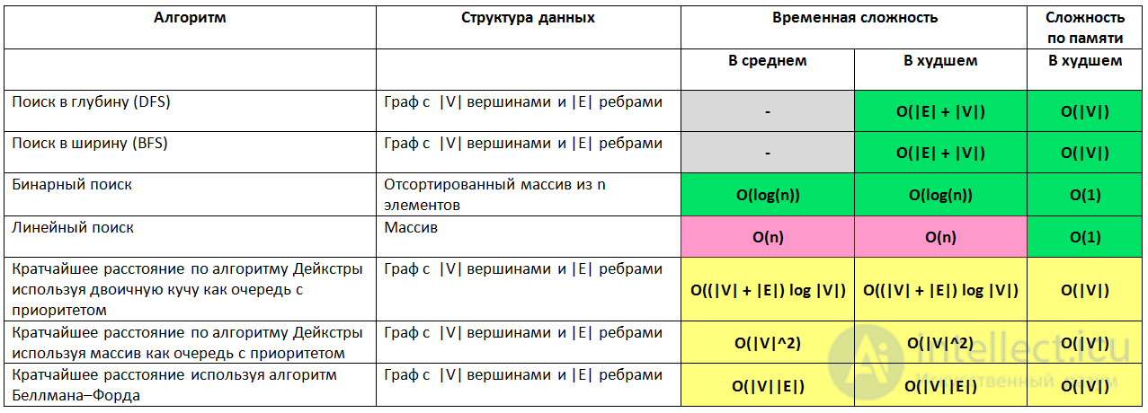
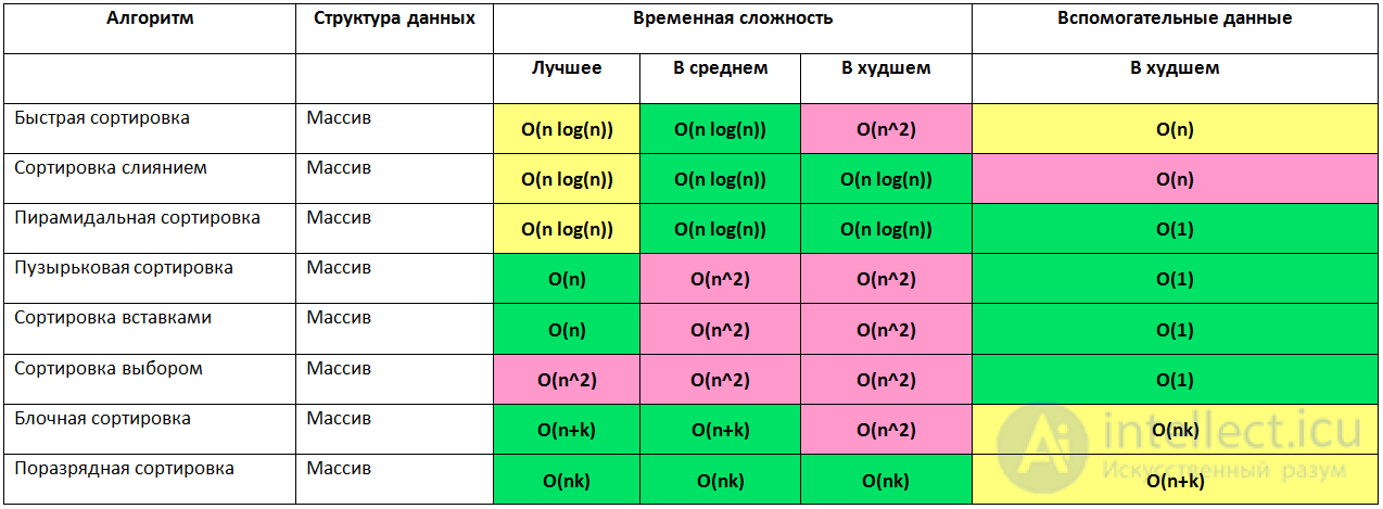
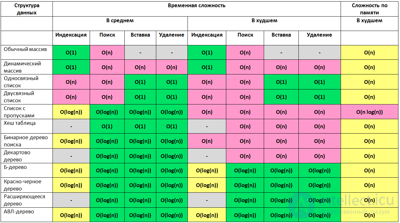
Average complexity describes the expected performance of an algorithm. It sometimes involves calculating the probability of each scenario. Below is a cheat sheet of the time and space complexity of typical algorithms.
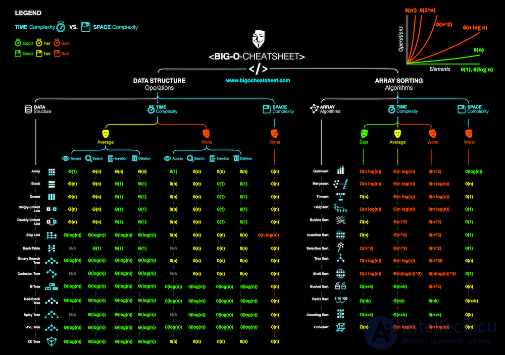
Big O Cheatsheet for Common Algorithms
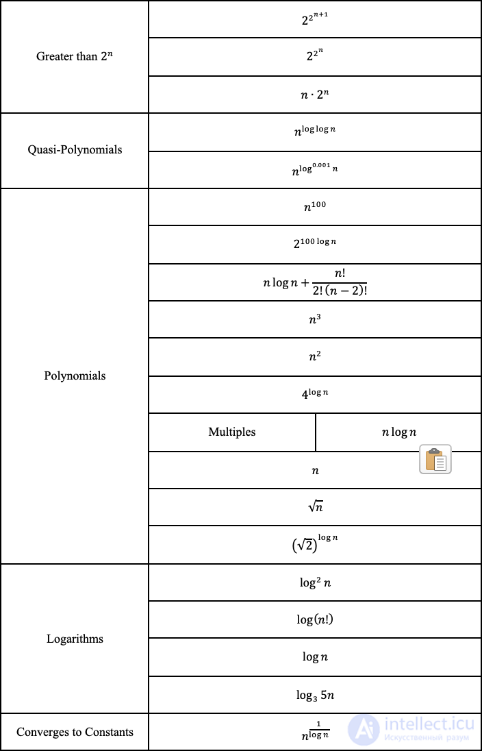
Examining the functions, we can start by ranking the following polynomials from most to least complex according to rule 3, where the square root of n is simply n to the power of 0.5.

Then, applying rules 2 and 6, we get the following. A logarithm with base 3 can be converted to one with base 2 (log base conversions). A logarithm with base 3 still grows slightly slower than one with base 2, and therefore ranks after it.

The rest may seem a bit complicated, but let's try to be a little more careful and see how all of them can be arranged.
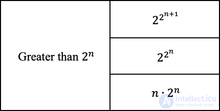
First of all, 2 to the power of 2 to the power of n is greater than 2 to the power of n, and the +1 increases it even further.
For the power of log (n) base 2 to equal n, we can transform the following. The logarithm of 0.001 grows a little more than a mere constant, but less than almost everything else.
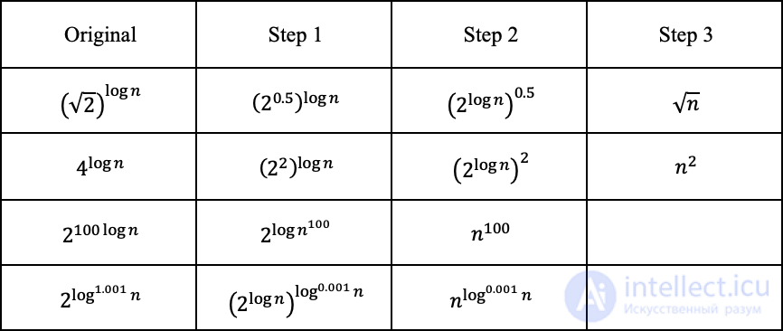
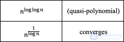
The expression with n to the power of log (log (n)) is actually a variation of a quasi-polynomial (quasi-polynomial), which is larger than a polynomial but smaller than an exponential. Since log (n) grows slower than n, its complexity is slightly smaller. The expression with the reciprocal logarithm converges to a constant, since 1 / log (n) diverges to infinity.
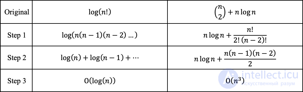
Factorials can be represented by multiplication and can therefore be converted into additions outside the logarithmic function. «N choose 2» can be converted into a polynomial with a cubic term being the largest.
And finally, we can rank the functions from most complex to least complex.
The idea discussed below is generally not accepted by most programmers in the world. Voice it in interviews at your own risk. There have been cases when people failed a Google interview because they questioned the necessity of the notation.
Since we learned earlier that the worst-case time complexity for quicksort is O (n²), while for merge sort it is O (n * log (n)), then merge sort should be faster, right? Well, you've probably guessed that the answer is no. To demonstrate this, I posted this example here at trinket.io (https://trinket.io/python/87a3166026). It compares the time for quicksort (quick sort) and merge sort (merge sort). I was only able to test it on arrays up to 10000 values in length, but, as you can see, the time for merge sort grows faster than for quicksort. Despite quicksort having a worse complexity of O (n²), the probability of that occurring is actually low. When it comes to increasing speed, quicksort has a higher speed than merge sort, which is bounded by a complexity of O (n * log (n)); quicksort ends up with better performance on average.
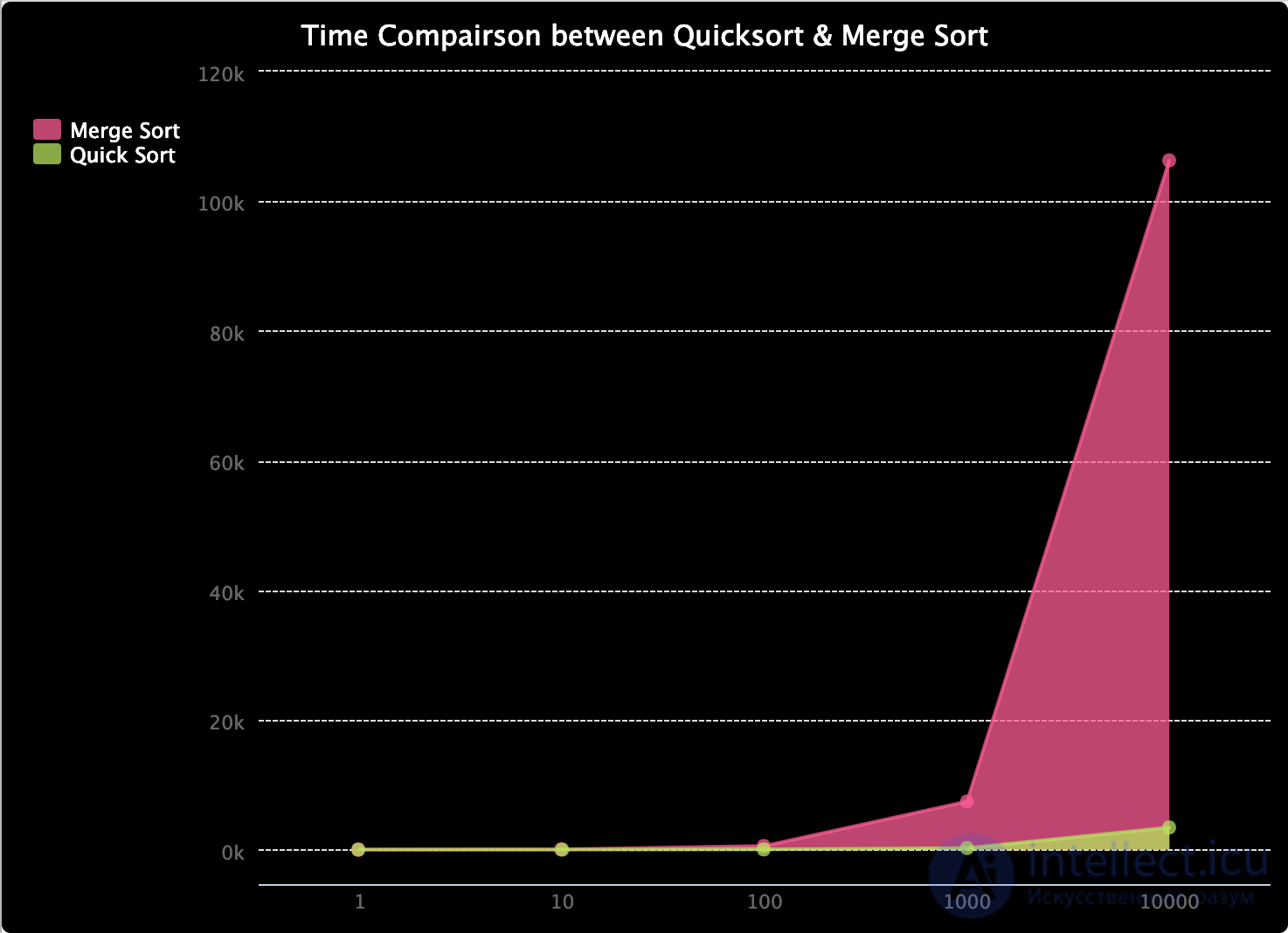
I also made a graph to compare the ratio between the times they take, since this time difference is hard to see at lower values. And, as you can see, the percentage of time required for quicksort decreases very quickly.
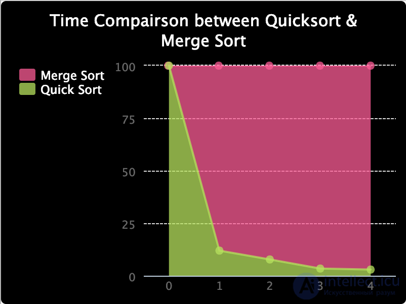
The moral of this story is that Big O notation is just a mathematical analysis that gives insight into the resources consumed by an algorithm. Practical results may vary. But, as a rule, it is good practice to try to reduce the complexity of our algorithms.
Часть 1 Analysis and Estimation of Algorithm Complexity: Big O and Complexity Functions
Часть 2 Assessing the complexity of algorithms - Analysis and Estimation of

Comments