
Lecture
Classification of Numerical Algorithms
Before we begin, we need to formalize the notion of algorithm complexity – a certain countable sequence of
actions. We will measure the complexity of an algorithm by a certain value that allows us to characterize the algorithm from the standpoint of its practical applicability. The smaller this value, the greater the feasibility of using the given algorithm.

Definition 1. By the complexity of an algorithm we mean the number of operations performed on elements of some finite set in the course of the algorithm. As a synonym for the complexity of an algorithm, we will also use the term algorithmic effort.
It follows immediately from our definition that the notion of complexity is not unambiguous and depends on the choice of the finite set over which the computations are performed. There are two approaches to choosing the set of operands — the first is based on fixing some mathematical object, for example, a group or a ring. The second approach is based on fixing the register length of the computing device that will implement the given algorithm. The first approach is simpler, more universal, and adopted in mathematical research; the second approach is tied to the computing device, more precise, and allows one to estimate
the complexity of the algorithm in clock cycles of the computing device. We will use the first approach, leaving the detailed analysis to software developers.
In both cases, some parameter n is considered, characterizing the set whose elements the algorithm operates on. The complexity of the algorithm is represented as a function of n.
Let n > 0 be an arbitrary integer or real variable.
Recall that the symbol O (f(n)) denotes a function such that
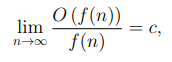
where c > 0 is some constant. Consider the function

of real variables  an integer or real variable.
Definition 2. Let f(n) — be a function specifying the complexity of an algorithm, the function L(x, z, n) defined by equality (1), the values x, z
fixed and  . We will use the following terminology.
1. The function f(n) is called polynomial if

2. The function f(n) is called exponential if

3. The function f(n) is called subexponential if

Let us also consider special cases.
4. If f(n) = O (1), or equivalently, z = 0 for any value of x, then f(n) is called a constant.
5. If f(n) = O (n) is exponential at z = 1, then f(n) is called the complexity of total (exhaustive) search.
As can be seen from this definition, a subexponential function occupies an intermediate position between polynomial and exponential functions. Indeed, for fixed values of z and n > 1 we obtain

.
Here we implicitly use the fact that for fixed values of z, n the function L(x, z, n) is a monotonically non-decreasing function.
Let us note one feature that arises when solving cryptographic problems. All the problems we consider necessarily have a
solution whose search can be reduced to enumerating all elements of some finite set characterized by an integer parameter n. Consequently, the maximum complexity of solving such a problem is determined by the complexity of total search, that is O (n).
However, in practical applications the value of the parameter n is so large that using total search does not allow
finding a solution in a reasonable time, even using the most productive computing resources available. In this regard, our
task reduces to finding algorithms whose complexity is less than that of total search.
Let us note that the existence of a polynomial, that is, fast algorithm for solving the problems we consider is, rather, a pleasant exception than the rule. Problems that have polynomial algorithms for their solution are extremely few; we list most of them below:
For the remaining problems we consider, the achievable minimum complexity is the existence of a subexponential algorithm.
Now let us consider yet another way of classifying algorithms. It is traditionally customary to divide all algorithms into deterministic
and probabilistic ones. For a deterministic algorithm, the complexity estimate is computed unambiguously, whereas for a probabilistic algorithm the complexity estimate is computed under certain assumptions, which can substantially affect the results obtained. Let us give some examples and explain the above.
Definition 3. An algorithm is called deterministic if, after a fixed number of steps (operations on elements of a finite set), the result of this algorithm's operation is always a solution to the stated problem. Note that the word «always» in this definition is
essentially important.
Definition 4. We will call an algorithm probabilistic if one of the following statements holds
In fact, one and the same algorithm can be regarded both as deterministic and as probabilistic, depending on our interpretation of this term, or on an attempt to minimize its complexity.
Let us consider the following example. Suppose we have an urn containing n balls – one red and n − 1 black balls. We can
draw balls from the urn without returning them. Our task is to draw the red ball.
If we draw all n balls from the urn one after another, then a red ball will necessarily be among them, hence we obtain a deterministic algorithm. The complexity of this algorithm equals n draws of a ball from the urn.
Now let us describe a variant of solving the same problem using a probabilistic algorithm satisfying the first statement of our
definition.
Let us fix the number of attempts to draw a ball from the urn and denote it by the symbol k. In this case, the probability of a successful termination of the algorithm, in other words, the probability that we will not draw k black balls in a row, will be equal to  for small values of k.
Thus, if we want to have a polynomial algorithm, we choose  , in which case the probability of its successful termination is small and equal to
l . It is obvious that when k = n we obtain the deterministic algorithm described earlier, since the probability of its successful termination equals one.
Let us fix the probability of successful termination of the algorithm and denote it by the symbol p, 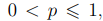 , then the average number of steps required for the algorithm to terminate successfully equals pn. Thus, fixing the success probability leads to a definition of the algorithm's complexity. If we set the probability equal to one, we obviously obtain that the average number of steps of the algorithm (draws of a ball from the urn) equals n. This is the second variant of a probabilistic algorithm in our definition.
A third variant of the algorithm in our definition can be obtained if we return the drawn black balls back to the urn. In this case there is a probability that we will never draw a red ball, that is, never complete execution of the algorithm.
Summarizing the above, note that we could initially define the notion of algorithm complexity as a function of two arguments —
the number of steps it performed and the probability of the algorithm's successful termination. However, such an approach to studying computational effort is not
generally accepted. Further on, unless stated otherwise,
we will estimate the complexity of probabilistic algorithms under the assumption that the probability of their successful termination is at least 1/2
We will begin the exposition with the simplest questions and consider the set of integers .

The set of integers forms a ring with respect to the operations of addition and multiplication. Let us introduce the operation of division on this set.
Definition 1.1. Let a, b be integers. We say that a divides b and write a|b if there exists an integer d such that ad = b.
It is well known that the division operation cannot be defined for two arbitrary integers a, b. It is easy to give an example, for instance, the number 3 does not divide the number 7, because it is impossible to find an integer d such that 3d = 7.
On the other hand, we can introduce another operation — the operation of division with remainder, which is defined for any pair of integers
a, b. We will need the following lemma.
Lemma 1.1. Let a, b be integers, then there exist unique integers q, r such that

Proof. Without loss of generality, assume that a > 0. Then there exists a largest integer q such that aq 6 b and b < a(q+1).
Denoting r = b − aq, we obtain the inequality 0 6 r < a and the representation (1.1). Suppose the representation (1.1) is not unique. Then there exist integers q1, r1 such that the equalities b = aq1 + r1 and aq + r = aq1 + r1 hold.
From the last equality it follows that a|(r1 − r). From the definition of the numbers r, r1 it follows that |r1 − r| < a. Thus, r1 − r = 0 and r1 = r, q1 = q. The lemma is proved.
Definition 1.2. Let a, b be integers. We will call the integer r  the remainder of dividing b by a, if
the representation (1.1) holds, or, equivalently, a|(b − r).
Algorithms:
Let us introduce one of the fundamental concepts in algebra and number theory,
namely, the concept of a residue modulo an integer.
Definition 2.1. Let a, b be integers, and m > 0 a natural number. We say that the numbers a and b are congruent modulo m and write  , if m|(a − b) or, equivalently, a = b + km for some integer value k.
From Definition 2.1 it follows that the solutions of the congruence 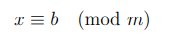 are all integers of the form b + km, where k is some integer.
These numbers form a class of numbers modulo m.
Definition 2.2. Any number from the class  will be called a residue modulo m. A residue x satisfying
the inequality  will be called the least non-negative residue. Let us take one representative from each class modulo m – the least non-negative residue. It is easy to see that there are exactly m such residues in total, and they are all distinct.
Definition 2.3. We will call a complete system of residues the set of all least non-negative residues modulo m.
Further on we will also need another way of defining representatives of residue classes, based on the absolute value
of the representative.
Definition 2.4. We will call x the absolutely least residue modulo m if it satisfies the inequality
1. 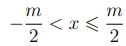 for even m;
2. 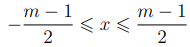 for odd m.
Definition 2.5. Similarly to Definition 2.3, we will call a complete system of absolutely least residues – the set of all absolutely least residues modulo m.
Algorithms:
Let us formalize our knowledge of polynomials: we will introduce the formal notion of a polynomial in one variable, define for polynomials the operations of addition, multiplication, and division with remainder, and show that for polynomials one can also prove the theorem on unique factorization.
We will denote by the symbol  an arbitrary commutative ring with unity. As examples of such rings, we can consider the ring of integers
  , the ring
  of residues modulo an integer m. Since fields are also rings, as the ring
  we will consider the field of rational numbers
  the field of real numbers
  as well as the finite field
 which forms a complete system of residues modulo a prime number p.
The proof of the fact that the set indeed forms a field consists in verifying all the axioms and follows from the results of
the previous chapter.
Definition 3.1. Let U be an arbitrary commutative ring with unity, and let a, b be nonzero elements of the ring U. We shall say that a divides b and use the notation a|b or b ≡ 0 (mod a) if there exists an element d in the ring U such that ad = b. We shall call the element a a divisor of the number b.
It is obvious that for the ring of integers Z this definition coincides with the previously introduced Definition 1.1.
Definition 3.2. We shall call an element ε of the ring U invertible if it is a divisor of unity, that is, if there exists some element ε
−1 of the same ring such that  . To denote the inverse element we shall also use the notation 1 /ε.
With respect to the operation of multiplication, the invertible elements form a group. Indeed, if a, b are two invertible elements of the ring U, then
there exist elements 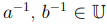 such that
 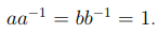 . Then, by virtue of the commutativity of the ring U, we obtain the equality

from which it follows that the element ab is also invertible. In the ring of integers Z there exist exactly two invertible elements, 1 and −1, which are also contained in any other ring. Arbitrary rings may contain more than two invertible elements; for example, in a field all elements other than zero are invertible. An invertible element ε divides any element of the ring U. Indeed, for any element a the equality holds 
.
Example 3.1. Consider the ring of residues  . Then the group of its invertible elements consists of the following residues Z

From Bezout's lemma, see Lemma 2.2, it follows that the invertible elements are precisely the residues coprime with the modulus. The number of
such numbers is determined by the value of Euler's function  and, according to Theorem 2.5, equals 8.
Let us give several important definitions and introduce the concept of the ring of polynomials in one variable U[x], which we shall use repeatedly in what follows.
Definition 3.3. Let U be an arbitrary commutative ring with unity and  an integer. We shall call a polynomial a(x) in one variable x the sum
We shall call the quantities 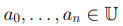 the coefficients of the polynomial, and the coefficient an the leading coefficient.
For some fixed value x ∈ U, we shall call the value of expression (3.1), belonging to the ring U, the value of the polynomial a(x).
We shall call the integer n the degree of the polynomial and denote it by the symbol deg a(x) = n. Polynomials of degree one shall be called linear.
As follows from the definition we have given, all elements of the ring U can be regarded as polynomials of degree zero. This statement is false only for zero, since for it we always have an = 0. Therefore
we shall additionally assume that deg 0 = −1.
Definition 3.4. A polynomial  , whose leading coefficient equals unity, is called monic1
.
Further, we shall denote by the symbol U[x] the set of polynomials in one variable x with coefficients from the ring U. Let
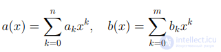
be two arbitrary polynomials. Without loss of generality, we shall assume that  . We define their sum by the equality
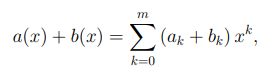
where the coefficients an+1, . . . , am are taken equal to zero. It is easy to see that  The «less than» sign arises in the case when the sum of the leading coefficients equals zero.
We define the product of polynomials by the equality

the equality also holds 
In Russian-language publications there is no established name for this polynomial. In the literature on number theory, the concept of a primitive polynomial is traditionally used, while in textbooks on algebra, the concepts of a monic, normalized, or reduced polynomial are used.
The operations we have introduced allow us to define on the set U[x] the structure of a commutative ring, whose unity and zero coincide
with the unity and zero of the ring U. The proof of this statement is carried out by verifying all the properties that a ring must satisfy.
We shall say that the polynomial
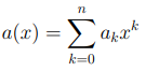
divides the polynomial b(x) if for some polynomial u(x) ∈ U[x] the equality a(x)u(x) = b(x) holds. Based on the definition of the operation of
multiplying polynomials, we immediately conclude that deg a(x) 6 deg b(x).
Note that if the leading coefficient an of the polynomial a(x) is invertible, then we can write the polynomial a(x) in the form
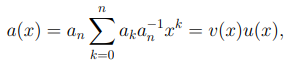
where  is a monic polynomial whose coefficients are defined by the equalities
  for k = 0, . . . , n.
Thus, a polynomial a(x) ∈ U[x] with an invertible leading coefficient can be represented as the product of a polynomial of degree zero and a monic polynomial of degree equal to the degree of the polynomial a(x). It is obvious that if the ring U is a field, then this holds
for any polynomial of positive degree.
Definition 3.5. A polynomial a(x) ∈ U[x] is called irreducible if the equality a(x) = u(x)v(x), where u(x), v(x) ∈ U[x], is possible only in the case when one of the polynomials u(x), v(x) has degree zero and, thus, is an element of the ring U. Solving the problem of checking whether a given polynomial is irreducible depends substantially on the ring over which the polynomial is considered. As is well known from a course in algebra, any polynomial
with coefficients from the field of complex numbers is reducible, since it factors into linear factors, see [5, ch.6, § 3]. For an arbitrary ring this is, of course, not true. However, we can prove a theorem on the factorization of polynomials analogous to the fundamental theorem of arithmetic for integers.
Let a(x) and b(x) be two polynomials from the ring U[x], where the leading coefficient of the polynomial a(x) is invertible; in particular, a(x)
may be a monic polynomial. Analogously to the ring of integers Z, we introduce the operation of division of polynomials with remainder and define two polynomials q(x), r(x) of the ring U[x] satisfying the equality b(x) = a(x)q(x) + r(x), deg r(x) < deg a(x). (3.2)
We shall call the polynomial q(x) the quotient of the division, and the polynomial r(x) – the remainder of the division of the polynomials. We give the definition of the operation of division with remainder by means of the following algorithm, often called the «school algorithm for polynomial division».
Algorithms:
Let us consider continued fractions of real numbers.
Definition 5.1. Let α be a real number. We will call the integer part of α, which we denote by the symbol  , the largest integer less than or equal to α. In the particular case, the integer part of an integer coincides with the integer itself.
Note that α can be either negative or positive.
For example  , while
In any case, the inequality  holds
holds
Let α0 be a real number and  . Let us define a sequence of real numbers α1, α2, . . . by the following recurrence relation

If αn turns out to be an integer, that is, the equality an = αn holds, we will consider that the sequence (5.1) terminates.
Writing equality (5.1) in the form 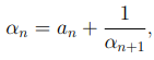 , we can express the number α0 as
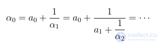
or, in general form,
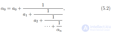
for an arbitrary index n.
To simplify the writing of equality (5.2) we will use the notation 
Definition 5.2. Let  be a real number. We will call representation (5.2)
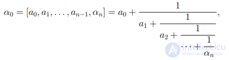
n = 1, 2, . . . the continued or chain fraction of the number α0. The elements of the sequence a0, a1, . . . we will call partial quotients,
and the elements of the sequence α1, α2, . . . complete quotients.
Note that from relation (5.1) and the inequality  it follows that the following inequalities hold

Algorithms:
In cryptographic applications, prime numbers play an important
role, being long-term parameters of cryptographic schemes
and being subject to attacks by adversaries in the first place. The lifetime of
public parameters is limited, which forces the developers of cryptographic schemes to generate, quite often, new prime numbers not previously used.
When generating prime numbers, additional conditions are usually imposed on them. As an example: according to the first edition of the Russian Federation standard for the digital signature GOST R 34.10-94, it is necessary to construct two prime numbers p, q
satisfying the conditions

The next edition of the standard imposes somewhat different conditions on the prime numbers p, q:

for some integer t satisfying the inequality  . When generating prime numbers, two questions typically arise.
1. How to construct a prime number with given constraints on the size of the number?
2. How to determine whether a given integer m is prime or composite?
These two questions are closely related: as soon as we have a criterion for testing primality, we can immediately propose an algorithm for constructing a prime number based on that criterion.
Moreover, the problem of testing primality of a number is related to the problem of factorization. The simplest way to check whether a number m is composite or not is to check the statement of Lemma 1.6, that is, to find out whether m has a prime divisor not exceeding  . If there is no such divisor, then the number m is prime. To enumerate all possible divisors we would need to perform about
  trial-division operations on the number m. For large values of m this procedure becomes impractical.
At the same time, trial division is often used to check whether a number has small divisors.
Let us give an algorithm for constructing a table of all prime numbers bounded above by some value b. Such tables will be used by us both for implementing the trial-division method and in some algorithms for factoring integers.
Algorithms:
Let us consider elementary methods for factoring a composite number m. These methods are fairly simple to describe, but have high computational cost, which prevents their use for factoring numbers used in practice. Nevertheless, the algorithms described can be used as components in more complex algorithms.
Throughout the chapter we will assume that m > 0 is an odd composite number. The question of how to determine whether the number m
is composite or prime was considered in the previous chapter.
Recall that by the problem of factorization we mean finding such prime numbers 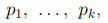 that the number m can be uniquely represented as the product
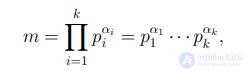
where αi are natural numbers. Such a representation, by virtue of the fundamental theorem of arithmetic, see Theorem 1.4, exists and is unique.
To find all prime divisors of the number m, we need to find two divisors of m, not necessarily prime ones, and then apply
the divisor-search procedure to each of the divisors found. Further on we will describe algorithms assuming that it is enough for us to find
two arbitrary divisors of the number m.
Algorithms:
Let us consider methods for solving the discrete logarithm problem
in the multiplicative group of the finite field Fp.
Definition 9.1. Let a prime number p and a residue a be given, whose order modulo p is equal to m, that is, 
Let a residue b be given, satisfying the congruence

The problem of determining the residue x (mod m) is called the problem of computing the index of the element b to the base a. In the cryptographic literature
the problem of computing the index has received the synonymous name: «the discrete logarithm problem».
For the residue x satisfying congruence (9.1), it is customary to use the notation

and call it the index, or discrete logarithm, of b to the base a.
From the definition given above and the statement of Lemma 2.3, it follows that the congruence (9.1) is solvable only when the residue b belongs to the set

that is, it is an element of the cyclic group generated by the element a. In this case, we will also say that the residue b belongs to the
set of possible powers of the residue a modulo p.
Before describing methods for solving the discrete logarithm problem, we shall describe the basic properties of indices.
Lemma 9.1. Let a prime number p and a residue a be given, whose exponent modulo p equals m, that is 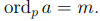 . Let a residue
b be given, belonging to the set of possible powers of the residue a modulo p. Then the following statements hold.
1. The congruence loga a ≡ 1 (mod m) holds.
2. Suppose that for the residue b the equality

holds, where α1, . . . , αn are arbitrary natural numbers, and the residues b1, . . .,
bn belong to the set A of possible powers of the residue a.
Then

3. The congruence  holds
holds
4. Let for the residues 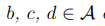 the following hold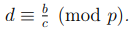

Proof. The first statement of the lemma holds by definition. To prove the second statement, consider the case where 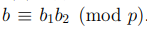 Since the residues b1 and b2 belong to the set of possible powers of the residue a, there exist residues x, y such that

Multiplying the residues b1 and b2, we obtain  (mod p).
Consequently, the congruence

holds. Generalizing this congruence to the case  , we obtain
the second statement of the lemma. It is easy to see that the third and fourth statements of the lemma are consequences of the second statement.
Example 9.1. It is particularly worth noting that the condition of
Lemma 9.1 requires that the residues b1, . . . , bn belong to the cyclic
subgroup generated by the residue a. Let us give an example in which violating this condition leads to a refutation of the lemma's statement.
Consider the equation

and note that 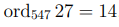 , that is, the residue 27 is not a primitive root and generates the multiplicative group

consisting of 14 elements. It is easy to see that a solution to our equation exists, and x = 8.
On the other hand, the equality  holds. Applying
the statement of Lemma 9.1 to find the unknown x, we must write the congruence

Since the residues 2, 5, and 13 do not belong to the group A, the indices 
 and
and  do not exist, and therefore the right-hand side of the congruence
(9.3) does not exist. Thus, we obtain a contradiction with the second statement of Lemma 9.1
Algorithms:

Comments