
Lecture
To obtain the models used for calculating (predicting) the operational failure rate λE of foreign-made components, the principles described in subsection 5.1 for components manufactured in CIS countries were applied.
The coefficients that enter into the mathematical models for calculating the operational failure rate of different classes of components can conventionally be divided into two groups (Table 6.1):
∙the first group of coefficients is common to the models of most classes (groups) of components and characterizes their operating modes and conditions, and the quality level of the components;
∙the second group of coefficients is included in the models of specific classes (groups) of components and characterizes the dependence of their operational failure rate on the design, functional and technological features of the components.
Table 6.1 Explanations of the coefficients used in the mathematical models
|
Symbol and |
Factors taken into account by the coefficient |
|
|
name of the coefficient |
||
|
|
||
|
Coefficients |
, included in the models for all classes of components |
|
|
Kt – the temperature |
Value of the component temperature |
|
|
mode coefficient |
||
|
|
||
|
KS – the electrical |
Electrical load – load factor KN |
|
|
mode coefficient |
||
|
|
||
|
KE – the operating |
Degree of severity of the operating conditions of the RED |
|
|
environment coefficient 1 |
||
|
KQ – the quality coefficient (analogous to the acceptance factor KP) |
Quality level – degree of severity of the requirements for control |
|
|
|
||
|
of quality and the acceptance rules for components under production conditions |
||
|
|
||
|
|
||
|
Coefficients, |
included in the models for integrated circuits (ICs) |
|
|
KL |
Duration of industrial production of the IC |
|
|
KF |
Functional purpose of the IC |
|
|
KI |
Manufacturing process of the IC |
|
|
Kkr |
Die complexity |
|
|
Kcorp |
Package type |
Coefficients included in the models for semiconductor devices
KK
KF
KD
KU
KI
KF
KS
Contact design of LF diodes
Functional purpose of the device
Maximum permissible power (current) load per the specifications
Coefficient depending on the ratio of the operating voltage to the maximum permissible value per the specifications (voltage load factor)
Coefficients included in the models for optoelectronic semiconductor devices
Maximum permissible peak forward current value per the technical documentation
Functional purpose of the device for laser diodes
Electrical load value for laser diodes
Components included in the models for resistors
|
KR |
|
Nominal resistance value |
|
KP |
|
Power dissipation value in the operating mode |
|
|
Components included in the models for capacitors |
|
|
KC |
|
Nominal capacitance value |
|
KSR |
|
Series resistance between the capacitor |
|
|
and the power bus (for oxide-semiconductor ca- |
|
|
|
|
pacitors) |
|
|
Note. 1 The selection of the coefficient KE is discussed in subsection 6.6. |
|
Below are the mathematical models that make it possible to predict the operational failure-free performance of certain classes and groups
components of foreign manufacture (Table 6.2). In systematizing and refining these models, the guidance of handbooks and standards from the USA, France and China [13–15] was used as a basis.
The calculation of the operational failure rate λE of individual IC groups is carried out according to the mathematical models of Table 6.2.
Table 6.2
|
|
Prediction models for the λE of ICs |
|
||
|
|
IC group |
Type of mathematical model |
Formula |
|
|
|
number |
|||
|
|
|
|
||
|
1. |
Digital microcircuits |
|
|
|
|
2. |
Analog microcircuits |
|
|
|
|
3. |
Programmable logic |
λE= (λkr ∙Kt + λcorp ∙KE)∙KQ ∙KL |
(6.1) |
|
|
integrated circuits |
||||
|
|
|
|||
|
(FPGA) |
|
|
||
|
4. |
Microprocessors |
|
|
|
|
5. |
Memory microcircuits |
λE= (λkr ∙Kt + λcorp ∙KE + λTs)∙KQ ∙KL |
(6.2) |
|
|
6. |
GaAs microwave microcircuits |
|
|
|
|
(GaAs MMIC) gallium arsenide |
λE= (λkr ∙Kt ∙KF + λcorp ∙KE)∙KQ |
|
||
|
ICs based on field-effect |
(6.3) |
|||
|
transistors and gold |
|
|
||
|
metallization |
|
|
||
|
7. |
VLSI (very-large-scale integration) |
λE = (λkrKI Kt Kkr + λkorp Kkorp )KEKQ + λel |
|
|
|
circuits (more than 60,000 logic |
(6.4) |
|||
|
cells – gates) |
|
|
||
|
8. |
SAW microcircuits |
λE = 2.1∙10-6∙KE ∙KQ |
(6.5) |
|
|
|
|
|
|
|
Note. λkr – failure rate of the IC due to the die; λcorp – failure rate of the IC associated with package failures; λTs – failure rate due to write/read cycles; λel – failure rate due to sensitivity to electrostatic discharge.
Model (6.1) applies to the following IC groups: digital bipolar-technology ICs; analog bipolar-technology ICs; programmable logic ICs (arrays) of bipolar technology; digital MOS-technology ICs; analog MOS-technology ICs; programmable logic MOS-technology ICs; bipolar-technology microprocessors; MOS-technology microprocessors.
Model (6.2) is used for the following groups of memory ICs: MOS-technology ROM; MOS-technology PROM; UV-erasable EPROM and EEPROM
with electrical erasure; MOS-technology dynamic RAM; MOS and combined-technology static RAM; bipolar-technology ROM, PROM; bipolar-technology static RAM.
Model (6.3) is used for the following groups of gallium arsenide ICs: digital; semiconductor microwave-range.
The failure rates λkr, λcorp for ICs (except for VLSI circuits) can be determined from the data in Tables 6.3–6.7.
Table 6.3 Failure rate values λkr for digital ICs, analog ICs and FPGAs
|
|
IC group |
λkr, × 10 –6 1/h |
Value of N |
|
|
1. |
Bipolar digital |
λkr = 0.0025 |
from 1 to 100 |
|
|
|
|
λkr = 0.000163∙N 0.6 |
from 101 to 60,000 |
|
|
2. |
Bipolar analog |
λkr = 0.010 |
from 1 to 100 |
|
|
|
|
λkr = 0.0174∙lnN – 0.06 |
from 101 to 10,000 |
|
|
3. |
FPGA |
λkr = 0.010 |
up to 200 |
|
|
λkr = 0.00216∙N 0.43 |
from 201 to 5000 |
|||
|
4. |
MOS digital |
λkr = 0.010 |
from 1 to 100 |
|
|
λkr = 0.00111∙N 0.54 |
from 101 to 60,000 |
|||
|
5. |
MOS analog |
λkr = 0.010 |
from 1 to 100 |
|
|
λkr = 0.0174∙lnN – 0.06 |
from 101 to 10,000 |
|||
|
|
|
|||
|
6. |
MOS-technology FPGA |
λkr = 0.00085 |
up to 500 |
|
|
|
|
λkr = 0.0022∙lnN – 0.0119 |
from 501 to 20,000 |
Note. N – the number of base cells (gates) for digital ICs and FPGAs, and the number of transistors for analog ICs.
Table 6.4
Failure rate values λkr for microprocessors
|
Word width, bits |
|
|
|
|
|
λkr, × 10 –6 1/h |
|
|
|
||||
|
|
|
Bipolar |
|
|
|
|
|
MOS |
|
||||
|
|
|
|
|
|
|
|
|
|
|
||||
|
up to 8 |
|
0.060 |
|
|
|
|
|
|
0.14 |
|
|
||
|
up to 16 |
|
0.12 |
|
|
|
|
|
|
0.28 |
|
|
||
|
up to 32 |
|
0.24 |
|
|
|
|
|
|
0.56 |
|
|
||
|
|
|
|
Values of λkr for memory ICs, × 10 –6 1/h |
|
|
Table 6.5 |
|||||||
|
|
|
|
|
|
|
||||||||
|
|
|
|
|
|
|
|
|
|
|
|
|
||
|
Memory capacity B, |
|
|
|
CMOS-technology ICs |
|
Bipolar ICs |
|||||||
|
|
|
|
PROM, |
Dynam- |
Stat- |
|
ROM, |
Stat- |
|||||
|
bits |
|
ROM |
|
|
|||||||||
|
|
|
EEPROM |
|
ic RAM |
ic RAM |
|
PROM |
ic RAM |
|||||
|
|
|
|
|
|
|
||||||||
|
|
|
|
|
|
|
|
|
|
|
|
|
|
|
|
up to 16 K |
|
0.00065 |
|
0.00085 |
|
0.0013 |
|
0.0078 |
|
0.0094 |
0.0052 |
||
|
16 < B ≤ 64 K |
|
0.0013 |
|
0.0017 |
|
0.0025 |
|
0.016 |
|
0.019 |
0.11 |
||
|
64 K < B ≤ 256 K |
|
0.0026 |
|
0.0034 |
|
0.0050 |
|
0.031 |
|
0.38 |
|
0.21 |
|
|
256 < B ≤ 1 M |
|
0.0052 |
|
0.0068 |
|
0.0100 |
|
0.062 |
|
0.75 |
|
0.42 |
|
|
Failure rate value λkr for gallium arsenide ICs |
Table 6.6 |
||||||||||||
|
|
|||||||||||||
|
|
|
|
|
|
|
||||||||
|
Microwave (MMIC) |
|
|
Digital, on MESFET transistors |
||||||||||
|
|
|
|
|
|
|
||||||||
|
IC complexity, number of |
|
λkr, × 10 –6 1/h |
|
IC complexity, number of |
λkr, × 10 –6 1/h |
||||||||
|
active elements |
|
|
|
|
|
active elements |
|
|
|
||||
|
1 to 100 |
|
4.5 |
|
|
|
|
1 to 1000 |
|
|
25 |
|||
|
101 to 1000 |
|
7.2 |
|
|
1001 to 10000 |
|
|
51 |
|||||
Table 6.7 Determination of the failure rate λcorp as a function of the number of leads n
|
|
Package type |
λcorp, × 10 –6 1/h |
|
1. |
Hermetic DIP, PGA, SMT |
λcorp = 2.8∙10 –4∙n 1.08 |
|
2. |
Glass-sealed DIP |
λcorp = 9.0∙10 –5∙n 1.51 |
|
3. |
Flat package with axial leads |
λcorp = 3.0∙10 –5∙n 1.82 |
|
4. |
Metal (can) |
λcorp = 3.0∙10 –5∙n 2.01 |
|
5. |
Non-hermetic DIP, PGA, SMT |
λcorp = 3.6∙10 –4∙n 1.08 |
Notes: 1. n – number of leads.
2.SMT – surface-mount packages: Small Outline (SO, SOIC, SOP, SOJ, WSOP, SSOP, TSOP, TSSOP, etc.); Flatpack (QFP, TQFP, etc.); Leaded Chip Carrier (LCC); Ball Grid Array (BGA), etc.
The failure rate associated with write/read cycles, λTs = 0 for all memory ICs except EEPROM with electrical erasure, for which λTs is determined from the data in Table 6.8.
Table 6.8 Calculation of the failure rate λTs for EEPROM
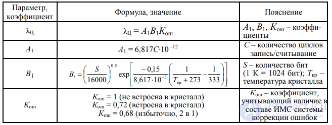
To obtain the failure rates λkr, λcorp, λel for VLSI ICs, use Table 6.9.
Table 6.9 Failure rates λkr, λcorp, λel for VLSI ICs
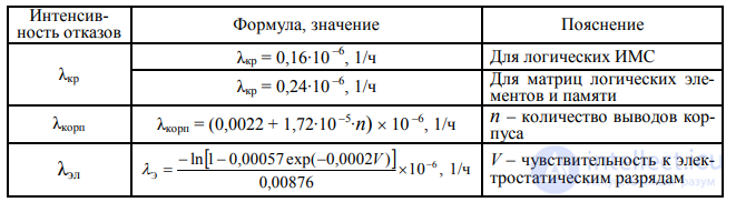
Note. In the formula for determining λel, when the value of V is unknown, use the value V = 0…1000 V.
The coefficient accounting for the effect of temperature, Kt, can be obtained from the models given in Table 6.10.
Table 6.10 Calculation of the mode coefficient Kt
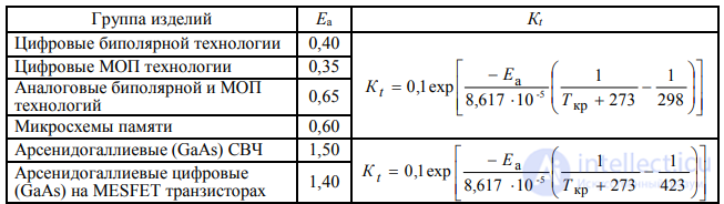
Note. Ea – activation energy, eV; Tkr – crystal temperature (the crystal-to-package junction temperature for Si devices, or the average channel temperature for GaAs devices), ºC.
The temperature Tkr is determined as
|
Tkr = Tcorp + Rkr-corpP, |
(6.6) |
where Tcorp – the IC package temperature, ºC;
Rkr-corp – the crystal-to-package thermal resistance, ºC/W;
P– the actual power dissipated by the IC in the operating mode.
As Tcorp, the maximum temperature should be taken, allowing for the IC's operation as part of the RES. If the value of P used in formula (6.6) cannot be determined, it is recommended to use information on the maximum dissipated power of the IC in question or of an equivalent IC. If the value of Rkr-corp is unknown, use the data for an equivalent IC, or Table 6.11.
|
|
|
Table 6.11 |
|
|
Selecting the value of Rkr-corp (for ICs in ceramic packages) |
|||
|
IC package |
Value of Rkr-corp (ºC/W) for a crystal area of |
||
|
> 9,29 mm2 |
≤ 9,29 mm2 |
||
|
|
|||
|
Type 2 (Dual-in-Line) |
11 |
28 |
|
|
Type 4 (Flat Package) |
10 |
22 |
|
|
Chip Carrier |
10 |
20 |
|
|
Pin Grid Array (PGA) |
10 |
20 |
|
|
Can (metal) |
– |
70 |
|
|
Organic Material Pack |
|
80 |
|
Coefficient KL, which accounts for the duration of industrial production of the IC, can be calculated using the model

where L – the duration, in years, of industrial production of ICs of this type.
The values of coefficient KF of model (6.3) and coefficient Kcorp of model (6.4) are selected from Tables 6.12 and 6.13.
Table 6.12 Selecting coefficient KF
|
Functional purpose |
KF |
|
|
Semiconductor microwave devices: |
1 |
|
|
low-noise, low-power |
||
|
high-power (> 100 mW) |
3 |
|
|
unknown |
3 |
|
|
Digital, all functional |
1 |
|
|
purposes |
||
|
|
|
|
|
Table 6.13 |
|
Coefficient Kcorp for VLSI circuits |
||
|
Type |
Values of Kcorp |
|
|
of package |
Hermetic |
Non-hermetic |
|
|
|
|
|
DIP |
1 |
1,3 |
|
PGA |
2,2 |
2,9 |
|
SMT |
4,7 |
6,1 |
|
|
|
|
Recommended values of coefficient KI of model (6.4):
0,55 – when manufactured using QML or QPL processes, 2 – when using other processes.
Coefficient Kkr of model (6.4) can be calculated using the formula

where Skr – the crystal area in cm2;
xs – the feature (topological) size in microns.
The values of coefficient KQ, which accounts for the effect of the IC manufacturing quality level, are given in Table 6.14 (all ICs except SAW microcircuits) and Table 6.15 (SAW microcircuits).
|
|
|
|
|
Table 6.14 |
|
|
|
Values of coefficient KQ for all ICs except SAW microcircuits |
|
|||
|
|
IC manufacturing quality level |
|
Approximate correspondence to the |
||
|
Characteristic per US reference books and standards |
KQ |
acceptance level in CIS countries |
|||
|
1. |
Class S per MIL-M-38510 |
0,25 |
“9” (OS) |
|
|
|
2. |
Class B per MIL-M-38510 |
1,0 |
“5” (VP, OVP) |
||
|
3. |
Class B1 per standard MIL-STD- |
2,0 |
“5” (VP, OVP) |
||
|
|
883, section 1.2.1 |
|
|
|
|
|
4. |
Quality level lower than class B1 |
3,1 |
“3” (QCD) |
|
|
|
5. |
Quality level lower than class B1 |
5,5 |
“1” (QCD) |
|
|
|
6. |
Commercial level, or level unknown |
10 |
“1” (QCD) |
|
|
|
|
|
|
|
Table 6.15 |
|
|
|
Values of manufacturing quality coefficient KQ for SAW integrated circuits |
||||
|
|
|
|
|
|
|
|
|
IC quality level |
|
|
|
KQ |
|
1. |
Tested through 10 temperature cycles (from –55 to +125°C) |
|
0,1 |
||
|
|
under electrical load (approximately corresponds to “5” acceptance) |
|
|||
|
|
|
|
|||
|
2. |
Lower quality level (approximately corresponds to “1” acceptance) |
|
1,0 |
||
Calculation of the operational failure rate λE of individual groups
of semiconductor devices (SD) is performed using the mathematical models of Table 6.16.
|
|
|
Table 6.16 |
|
|
|
Mathematical models for calculating λE of semiconductor devices |
||
|
|
Product group |
Type of mathematical model |
|
|
1. |
Low-frequency diodes |
λE = λB ∙ Kt ∙ KS ∙ KK ∙ KQ ∙ KE |
|
|
2. |
High-frequency diodes |
λE = λB ∙ Kt ∙ KF ∙ KD ∙ KQ ∙ KE |
|
|
3. |
Low-frequency bipolar transistors (frequency |
λE = λB ∙ Kt ∙ KF ∙ KD ∙ KS ∙ KQ ∙ KE |
|
|
below 200 MHz) |
|||
|
|
|||
|
4. |
Low-frequency field-effect transistors |
λE = λB ∙ Kt ∙ KF ∙ KQ ∙ KE |
|
|
(p- and n-channel silicon, frequency below 400 MHz) |
|||
|
|
|||
|
5. |
Unijunction transistors |
λE = λB ∙ Kt ∙ KQ ∙ KE |
|
|
6. |
High-frequency low- and medium-power bipolar |
λE = λB ∙ Kt ∙ KD ∙ KS ∙ KQ ∙ KE |
|
|
transistors, including low-noise ones, frequency |
|||
|
above 200 MHz, power below 1 W |
|
||
|
7. |
High-power high-frequency (microwave) bipolar transistors |
λE = λB ∙ Kt ∙ KF ∙ Km ∙ KQ ∙ KE |
|
|
high power, average power above 1 W |
|||
|
|
|||
|
8. |
High-frequency gallium arsenide field-effect |
λE = λB ∙ Kt ∙ KF ∙ Km ∙ KQ ∙ KE |
|
|
gallium, low and medium power |
|||
|
|
|||
|
9. |
High-frequency gallium arsenide field-effect |
λE = λB ∙ Kt ∙ KF ∙ Km ∙ KQ ∙ KE |
|
|
gallium, high power, frequency above 1 GHz |
|||
|
|
|||
|
10. |
High-frequency silicon field-effect transistors |
λE = λB ∙ Kt ∙ KQ ∙ KE |
|
|
11. |
Thyristors |
λE = λB ∙ Kt ∙ KD ∙ KS ∙ KQ ∙ KE |
|
|
|
Note. λB – base failure rate. |
|
|
The values of the base failure rate λB are given in Table 6.17. The coefficients Kt of the models in Table 6.16 are determined using Tables 6.18, 6.19.
|
Reference data for λB of semiconductor devices |
Table 6.17 |
|
|
|
|
|
|
|
Product group |
λB × 10 –6 1/h |
|
1. Low-frequency diodes: |
0,0038 |
|
general-purpose rectifier diodes |
|
|
high-power fast-recovery rectifier diodes |
0,025 |
|
high-power rectifier diodes (incl. Schottky) |
0,003 |
|
switching diodes |
0,001 |
|
protective diodes (suppressors) / varistors |
0,0013 |
|
current regulators |
0,0034 |
|
zener diodes |
0,002 |
|
2. High-frequency (microwave) diodes: |
0,22 |
|
IMPATT diodes |
|
|
Gunn diodes |
0,18 |
|
tunnel and backward diodes (including mixer |
0,0023 |
|
and detector diodes) |
|
|
PIN diodes |
0,0081 |
|
Schottky-barrier diodes (including detector diodes) |
0,027 |
|
varactors (varicaps) and charge-storage diodes |
0,0025 |
|
3. Low-frequency bipolar transistors |
0,00074 |
|
|
|
End of Table 6.17 |
|
|
|
Product group |
λB × 10 –6 1/h |
|
|
4. |
Low-frequency field-effect transistors: |
0,012 |
|
|
|
MOS (MOSFET) |
||
|
|
junction (JFET) |
0,0045 |
|
|
5. |
Unijunction transistors |
0,0083 |
|
|
6. |
High-frequency low- and medium-power bipolar |
0,18 |
|
|
transistors |
|||
|
|
|||
|
7. |
High-power microwave bipolar transistors |
per formula (6.9)1 |
|
|
8. Low- and medium-power high-frequency gallium arsenide field-effect |
0,052 |
||
|
transistors, power below 0,1 W, |
|||
|
frequency 1 < F < 10 GHz |
|
||
|
9. |
High-power microwave gallium arsenide field-effect |
per formula (6.10)2 |
|
|
transistors, frequency 4 ≤ F ≤ 10 GHz, power 0,1 ≤ F ≤ 6 W |
|
||
|
10. High-frequency silicon field-effect transistors: |
0,06 |
||
|
|
MOS (MOSFET) |
||
|
|
junction (JFET) |
0,023 |
|
|
11. Thyristors |
0,0022 |
||
|
|
Notes: 1 The failure rate value λB is calculated using the formula |
||
|
|
λB = 0,032∙e 0,354∙F + 0,00558∙P . |
(6.9) |
|
2 The failure rate value λB is calculated using the formula
|
λB = 0,0093∙e 0,429∙F + 0,486∙P, |
(6.10) |
|
where F – the operating frequency, GHz, |
|
|
P – the average output power (per the documentation), W. |
|
|
|
Table 6.18 |
Calculation of the mode coefficient Kt as a function of the junction
temperature for all semiconductor devices except high-power high-frequency bipolar transistors
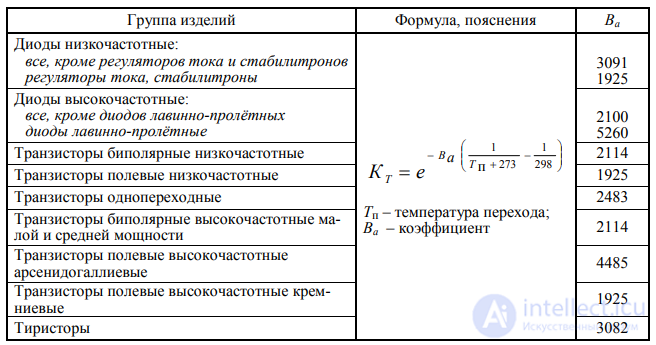
Calculation of the mode coefficient Kt as a function of the junction temperature for high-power high-frequency bipolar transistors
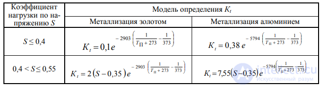
Note. S – the voltage electrical load coefficient; Tp – the peak junction temperature value, °C.
The junction temperature Tp (see Tables 6.18, 6.19) is calculated using the expression
|
Tp = Tokr + Rkr-okr∙P = Tcorp + Rkr-corp∙P, |
(6.11) |
where Tokr – the ambient temperature; °C;
Tcorp – the device package temperature, °C;
Rkr-okr – the “crystal – ambient” thermal resistance; °C/W; Rkr-corp – the “crystal – package” thermal resistance; °C/W;
P– the actual power dissipation of the device, W.
The thermal resistance values are taken from the device specification. Coefficients KK, KD, KF, KM and KS of the models in Table 6.16 are determined
using Tables 6.20–6.24.
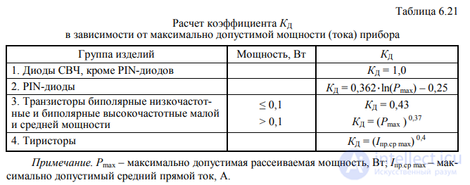
Table 6.22 Values of coefficient KF
depending on the functional purpose of the device
|
Product group |
Functional operating mode |
KF |
|
|
Microwave diodes, except varactors |
– |
1 |
|
|
Varactors |
Voltage-tuned |
0,5 |
|
|
Frequency multiplier |
2,5 |
||
|
|
|||
|
Low-frequency bipolar |
Linear amplification |
1,5 |
|
|
transistors |
|
|
|
|
Switching |
0,7 |
||
|
|
Small-signal switching |
0,7 |
|
|
|
|
|
|
|
|
Linear amplification (P < 2 W) |
1,5 |
|
|
Field-effect transistors |
Amplification (P ≥ 2 W): |
|
|
|
2 ≤ P < 5 W |
2 |
||
|
low-frequency |
|||
|
|
5 ≤ P < 50 W |
4 |
|
|
|
50 ≤ P < 250 W |
8 |
|
|
|
P ≥ 250 W |
10 |
|
|
High-power microwave bipolar |
Continuous mode |
7,6 |
|
|
transistors |
Pulsed mode |
KF = 0,06∙(D, %) + 0,4 |
|
|
High-frequency gallium arsenide |
Continuous mode |
4 |
|
|
field-effect transistors |
Pulsed mode |
1 |
Note. D – the reciprocal of the pulse duty cycle (fill factor), %.
Table 6.23 Calculation of coefficient KS as a function of the electrical load on semiconductor devices
|
Product group |
Load by |
KS |
Explanation |
|
|||
|
voltage S |
|
||||||
|
|
|
|
|
|
|
|
|
|
Low-frequency diodes, except voltage |
from 0 to 0.3 |
KS = 0.054 |
|
|
|
|
|
|
regulator diodes, current regulators and varistors, |
> 0.3 to1 |
KS = S 2.43 |
|
U rev.op |
|
||
|
protective diodes (suppressors) |
|
|
S = |
|
|
|
|
|
|
|
|
|
|
|
||
|
|
|
|
U rev.max |
|
|||
|
Voltage regulators, current regulators and vari- |
from 0 to 1 |
KS = 1 |
|
||||
|
stors, protective diodes (suppressors) |
|
|
|
|
|
||
|
|
|
|
|
|
|
|
|
|
Bipolar low-frequency transistors, |
|
KS = 0.045∙e 3.1∙S |
|
|
|
|
|
|
and bipolar high-frequency low- |
from 0 to 1 |
|
|
U CE.op |
|
||
|
and medium-power transistors |
|
|
S = |
|
|||
|
|
|
|
|
|
|||
|
Thyristors |
From 0 to 0.3 |
KS = 0.1 |
|
U CE.max |
|
||
|
> 0.3 to 1 |
KS = S 1.9 |
|
|
|
|
|
|
Note. Urev.op – steady-state reverse operating voltage; Urev.max – maximum reverse voltage permitted by the specification; Uce.op – operating collector-emitter voltage; Uce.max – maximum collector-emitter voltage permitted by the specification.
Table 6.24 Values of coefficient KM depending on the presence of matching circuits for high-frequency (microwave) transistors
|
Nature of matching in the electrical circuit |
Value of KM |
|
Matched at input and output |
1 |
|
Matched at input |
2 |
|
Not matched, or the nature of matching is unknown |
4 |
The voltage load factor S (see Table 6.23) is determined as
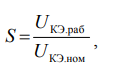 (6.12)
where UCE.op – collector-emitter voltage in the operating mode;
UCE.nom – maximum permissible (rated) collector-emitter voltage.
Values of the quality-level coefficient KQ are selected from Tables 6.25–6.27.
Table 6.25 Quality-level influence coefficient KQ (low-frequency diodes; transistors: bipolar low-frequency, field-effect low-frequency, unijunction; thyristors)
|
Quality level per MIL-S-19500 |
|
KQ |
|
Correspondence to domestic |
|
|
|
|
acceptance types |
|||
|
|
|
|
|
|
|
|
JANTXV |
|
0.7 |
“7”, “9” |
||
|
JANTX |
|
1.0 |
“5” |
||
|
JAN |
|
2.4 |
“3” |
||
|
Lower quality level |
5.5 |
“1” |
|||
|
Plastic |
|
8 |
|
“1”, plastic packages |
|
|
Quality level unknown |
10 |
|
|
||
|
|
|
|
|
|
Table 6.26 |
|
Quality-level influence coefficient KQ (microwave diodes) |
|||||
|
Quality level per |
KQ |
|
|
|
Correspondence to domestic |
|
MIL-S-19500 |
Microwave diodes, except |
|
Schottky |
|
acceptance types |
|
|
Schottky diodes |
|
diodes |
|
|
|
JANTXV |
0.5 |
|
0.5 |
|
“9” |
|
JANTX |
1 |
|
1 |
|
“5” |
|
JAN |
5 |
|
1.8 |
|
“3” |
|
Lower |
25 |
|
2.5 |
|
“1” |
|
quality level |
|
|
|||
|
|
|
|
|
|
|
|
Plastic |
50 |
|
– |
|
“1”, plastic packages |
Table 6.27 Quality-level influence coefficient KQ (bipolar high-frequency transistors, field-effect high-frequency transistors)
|
Quality level per MIL-S-19500 |
KQ |
Approximate correspondence to domes- |
|
|
tic acceptance types |
|||
|
|
|
||
|
JANTXV |
0.5 |
“9” |
|
|
JANTX |
1.0 |
“5” |
|
|
JAN |
2.0 |
“3” |
|
|
Lower quality level |
5.0 |
“1” |
|
|
Plastic |
8 |
“1”, plastic packages |
|
|
Quality level unknown |
10 |
– |
The selection of values of coefficient KE, which accounts for the severity of operating conditions, is discussed in subsection 6.7.
The operational failure rate λE of individual groups of optoelectronic semiconductor devices is calculated using the mathematical models included in Table 6.28.
Table 6.28 Models for calculating λE of optoelectronic semiconductor devices
|
Product group |
Type of mathematical model |
|
|
|
|
Photodetectors, optocouplers, semiconductor emit- |
λE = λB· Kt · KQ · KE |
|
ters, alphanumeric displays |
|
|
Laser diodes |
λE = λB ·Kt · KI · KF · KP · KQ ·KE |
|
Note. λB – base failure rate. |
|
Values of the base failure rate λB are given in Table 6.29.
|
|
Reference data λB for individual groups |
Table 6.29 |
|
|
|
|
|
|
of optoelectronic semiconductor devices |
|
|
|
|
|
|
|
Product group |
λB × 10 –6 1/h |
|
1. |
Transistor photodetectors (phototransistors) |
0.0055 |
|
2. |
Diode photodetectors (photodiodes) |
0.004 |
|
3. |
Single diode optocouplers |
0.0025 |
|
4. |
Single transistor optocouplers (including Darlington pair) |
0.013 |
|
5. |
Single resistor optocouplers |
0.0064 |
|
6. |
Binary diode optocouplers |
0.0033 |
|
7. |
Binary transistor optocouplers (including Darlington pair) |
0.017 |
|
8. |
Binary resistor optocouplers |
0.0086 |
|
9. |
Infrared emitting diodes |
0.0013 |
|
10. Light-emitting diodes |
0.00023 |
|
|
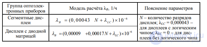
11. Segment displays |
per Table 6.30 1 |
|
|
12. Diode-matrix displays |
per Table 6.30 1 |
|
|
13. Laser diodes (type of semiconductor emitting |
|
|
|
material): |
|
|
|
|
GaAs / AlGaAs |
3.23 |
|
|
InGaAs / InGaAsP |
5.65 |
Note. 1 Models for calculating the base failure rate λB of segment displays and diode-matrix displays are given in Table 6.30.
Table 6.30 Base failure rate λB of segment displays and diode-matrix displays
Coefficients Kt, , KF and KS of the models in Table 6.28 are determined using Tables 6.31–6.33.
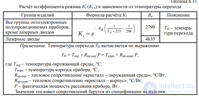
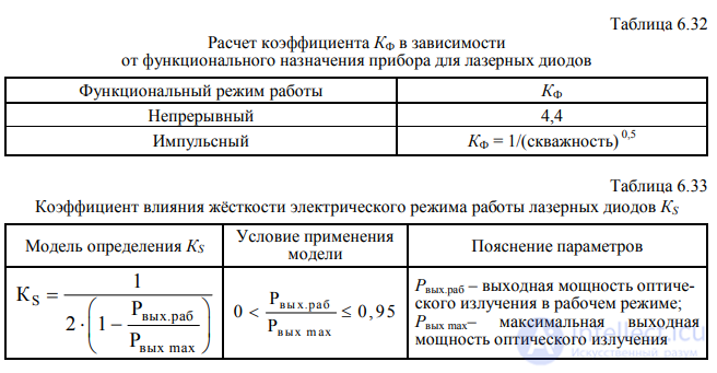
The forward-current influence coefficient KI is determined from the model
Table 6.34 Quality-level influence coefficient KQ for laser diodes
|
Quality level |
KQ |
|
|
Hermetic package |
1 |
|
|
Non-hermetic, coated |
1 |
|
|
Non-hermetic, uncoated |
3.3 |
|
|
Degree of package hermeticity not estab- |
5 |
|
|
lished, quality level unknown |
||
|
|
|
KI = I 0.68, |
(6.13) |
where I – peak value of forward current, A (I < 25 A).
Values of the quality-level coefficient KQ are selected
depending on the group of op- toelectronic devices per Tables 6.34, 6.35.
Table 6.35 Values of the manufacturing-quality influence coefficient KQ for optoelectronic semiconductor devices, except laser diodes
|
Quality level per MIL-S-19500 |
KQ |
Approximate correspondence |
|
|
to domestic acceptance types |
|||
|
|
|
||
|
JANTXV |
0.7 |
“7” |
|
|
JANTX |
1.0 |
“5” |
|
|
JAN |
2.4 |
“3” |
|
|
Lower quality level |
5.5 |
“1” |
|
|
Plastic |
8 |
“1”, plastic packages |
|
|
Quality level unknown |
10 |
– |
The selection of values of the operating-environment coefficient KE is discussed in sub- section 6.7.
For all groups and types of resistors, the operational failure rate λE is calculated using the model
|
λE = λB · Kt ·KP · KS ·KE ·KQ, |
(6.14) |
where λB – base failure rate of resistors of the given group (Table 6.36).
|
|
|
Table 6.36 |
|
|
Reference data for determining the parameters of model (6.14) |
|
|
|
|
|
|
|
Resistor group |
λB, × 10 –6 1/h |
|
1. |
Fixed composition insulated resistors (RC, RCR) |
0.0017 |
|
2. |
Fixed film insulated resistors (RL, RLR) |
0.0037 |
|
3. |
Fixed high-stability film resistors (RN) |
0.0037 |
|
4. |
Fixed unencased (chip) film resistors (RM) |
0.0037 |
|
5. |
Fixed power film resistors (RD) |
0.0037 |
|
6. |
Fixed film resistor networks (RZ) |
0.0019 |
|
7. |
Fixed precision wirewound resistors (RB, RBR) |
0.0024 |
|
8. |
Fixed power wirewound resistors (RW, RWR) |
0.0024 |
|
9. |
Fixed power wirewound resistors, chassis- |
0.0024 |
|
|
mounted (RE, RER) |
|
|
10. |
Insulated thermistors (RTH) |
0.0019 |
|
11. |
Variable wirewound trimmer resistors (RT, RTR) |
0.0024 |
|
12. |
Variable precision wirewound resistors (RR, RA) |
0.0024 |
|
13. |
Variable semi-precision wirewound resistors (RK) |
0.0024 |
|
14. |
Variable power wirewound resistors (RP) |
0.0024 |
|
15. |
Variable non-wirewound resistors (RJ, RJR) |
0.0037 |
|
16. |
Variable composition resistors (RV) |
0.0037 |
|
17. |
Variable precision non-wirewound resistors (RQ) |
0.0037 |
|
18. |
Variable non-wirewound film resistors (RVC) |
0.0037 |
Note. The parentheses give the abbreviations used abroad for the corre- sponding resistor groups.
54
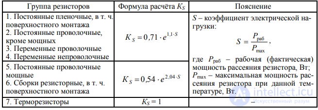
Coefficients Kt, KS and KQ of model (6.14) are determined using Tables 6.37–6.39.
Table 6.37 Calculation of coefficient Kt depending on the resistor case temperature
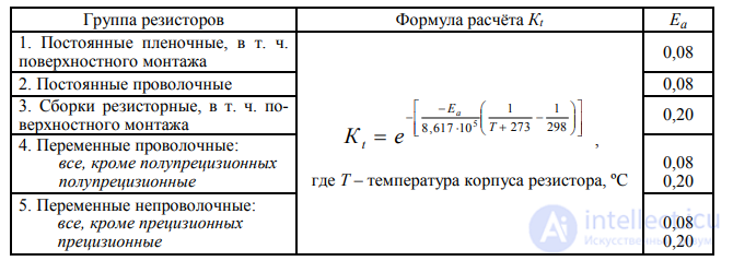
Note. For low-power resistors (maximum dissipated power Pmax < 1 W) the package temperature T is taken equal to the ambient temperature.
Table 6.38 Calculation of coefficient KS as a function of the resistor's electrical load
The coefficient KP, which accounts for the effect of dissipated power, is determined by the formula
|
KP = (Prab) 0,39, |
(6.15) |
where Prab – dissipated power of the resistor in the operating mode, W.
The selection of values of the operating-environment factor KE is discussed in Section 6.7.
For all groups and types of capacitors, the operational failure rate is calculated using the model
|
λE = λB · Kt · KC · KS ·KSR ·KE ·KQ , |
(6.16) |
where λB – base failure rate (Table 6.40).
Table 6.40 Reliability characteristics and reference data for individual capacitor groups
|
|
|
|
Group abbreviations |
λB, |
Ea |
|
|
|
Product group |
General Specifications |
of capacitors, |
|||
|
|
used |
× 10 –6 1/h |
|
|||
|
|
|
|
abroad |
|
|
|
|
1. |
Paper / with organic |
MIL-PRF-19978 |
CP, CA, CZ, CZR, |
|
|
|
|
MIL-PRF-39022 |
0,00051 |
0,35 |
||||
|
|
and synthetic dielectric |
MIL-PRF-55514 |
CQ, CQR, CH, |
|||
|
|
|
MIL-PRF-83421 |
CHR, CRH |
|
|
|
|
|
|
|
|
|
|
|
|
2. |
Mica |
MIL-PRF-39001 |
CM, CMR, CB |
0,00076 |
0,35 |
|
|
3. |
Glass |
MIL-PRF-23269 |
CY, CYR |
0,00076 |
0,35 |
|
|
4. |
Ceramic, fixed capaci- |
MIL-PRF-20 |
CC, CCR |
0,00099 |
0,35 |
|
|
|
tance, temperature-compensating |
|
|
|
|
|
|
5. |
Ceramic, fixed |
MIL-PRF-123 |
CK, CKR |
0,00099 |
0,35 |
|
|
6. |
capacitance |
MIL-PRF-39014 |
||||
|
7. |
Ceramic, fixed capaci- |
MIL-PRF-55681 |
Chip CDR |
0,002 |
0,35 |
|
|
|
tance, surface-mount |
|
|
|
|
|
|
8. |
Ceramic, variable |
MIL-PRF-81 |
CV |
0,0079 |
0,15 |
|
|
9. |
capacitance (trimmers) |
|||||
|
|
|
|
|
|||
|
10. |
Solid electrolytic (oxide-semiconductor) |
MIL-PRF-39003 |
CSR |
0,0004 |
0,15 |
|
|
11. |
Solid electrolytic (oxide-semiconductor), |
MIL-PRF-55365 |
Chip CWR |
0,00005 |
0,15 |
|
|
|
surface-mount |
|||||
|
|
|
|
|
|
||
|
12. |
Solid tantalum (sintered-anode) |
MIL-PRF-39006 |
CL, CLR |
0,0004 |
0,15 |
|
|
13. |
Oxide-electrolytic |
MIL-PRF-39018 |
CU, CUR, CE |
0,00012 |
0,35 |
|
|
|
aluminum |
|||||
|
|
|
|
|
|
||
|
14. |
Variable, piston-type |
MIL-PRF-14409 |
PC |
0,006 |
0,35 |
|
|
|
tubular trimmer capacitors |
|
|
|
|
The coefficient Kt, which accounts for the effect of elevated temperature, is calculated using the model

where Ea – activation energy, eV (see Table 6.40);
T– capacitor package temperature, ºC (taken equal to the maximum operating temperature of the electronic device).
The coefficients KC and KS of model (6.16) are determined using Tables 6.41, 6.42.
Table 6.41 Calculation of coefficient KC as a function of the capacitor's rated capacitance

Table 6.42 Calculation of coefficient KS as a function of the capacitor's electrical load by voltage
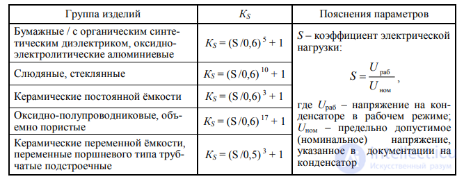
Note. Urab is the sum of the applied direct voltage and the maximum (peak) alternating voltage.
The values of the series-resistance influence coefficient KSR are chosen using the data in Table 6.43.
In this table R/Urab – the ratio of the active series resistance R between the capacitor and the power source to the working voltage on the capacitor Urab.
The values of the quality-level coefficient KQ are chosen from Table 6.44.
Table 6.43 Series-resistance influence coefficient KSR
|
R/Urab, Ohm / V |
KSR |
|
> 0,8 |
0,66 |
|
> 0,6 to 0,8 |
1 |
|
> 0,4 to 0,6 |
1,3 |
|
> 0,2 to 0,4 |
2 |
|
> 0,1 to 0,2 |
2,7 |
|
0 to 0,1 |
3,3 |
|
|
|
|
Table 6.44 |
|
|
Values of the manufacturing-quality coefficient KQ for capacitors |
||||
|
Quality level |
|
|
Approximate |
|
|
|
Designation |
|
correspondence |
|
|
|
KQ |
to domestic |
||
|
Acceptance characteristics of products |
of level |
|||
|
quality types |
||||
|
|
quality |
|
acceptance |
|
|
|
|
|
||
|
|
|
|
|
|
|
Products with Military acceptance under a published |
D |
0,001 |
– |
|
|
quality level, manufactured in accordance with |
C |
0,01 |
– |
|
|
MIL-PRF-39003, MIL-PRF-55365 |
|
|
|
|
|
B |
0,03 |
– |
||
|
|
||||
|
Products with Military acceptance under a published |
S |
0,03 |
“9” |
|
|
quality level, manufactured in accordance with |
|
|
|
|
|
R |
0,1 |
“9” |
||
|
MIL-PRF-19978, MIL-PRF-39022, MIL-PRF-55514, |
||||
|
MIL-PRF-83421, MIL-PRF-39001, MIL-PRF-23269, |
|
|
|
|
|
P |
0,3 |
“7” |
||
|
MIL-PRF-20, MIL-PRF-39014, |
||||
|
|
|
|
|
|
|
MIL-PRF-55681, MIL-PRF-39006, MIL-PRF-39018 |
M |
1 |
“5” |
|
|
– |
L |
2 |
“3” |
|
|
Products with Military acceptance and an unpublished quality level |
3 |
“3” |
||
|
Products with a lower quality level |
|
10 |
“1” |
|
The values of the operating-environment factor KE are chosen in accordance with Section 6.7.
Table 6.45 gives approximate (averaged) values of the coefficient KE, for the equipment groups listed in Table 6.45. The averaging of the KE values was performed using data from the US military handbook [13] and the Chinese standard [15].
Table 6.45 Coefficient of the influence of operating-condition severity KE
|
|
|
Equipment group depending |
|||||||
|
Class (component group) |
on the operating conditions per Table 5.21 |
||||||||
|
|
|
ZR |
ZChR |
ZOV |
ZPN |
ZM |
ZMD |
BSK |
|
|
1. IC |
|
1 |
1,5 |
2 |
4 |
6 |
8 |
8 |
|
|
2. Semiconductor devices, including optoelectronic: |
|
|
|
|
|
|
|
||
|
low-frequency diodes (rectifier, |
1 |
1,2 |
2 |
6 |
7,5 |
9 |
13 |
||
|
pulse, zener diodes), except for high-frequency diodes |
|||||||||
|
and microwave |
|
|
|
|
|
|
|
||
|
high-frequency and microwave diodes |
1 |
1,1 |
1,5 |
2 |
4 |
5 |
4 |
||
|
transistors |
bipolar low-frequency, |
1 |
1,2 |
2,5 |
6 |
7,5 |
9 |
13 |
|
|
low-frequency field-effect transistors, uni- |
|||||||||
|
junction transistors |
|
|
|
|
|
|
|
||
|
transistors |
bipolar high-frequency and |
1 |
1,3 |
1,7 |
2 |
4 |
5 |
4 |
|
|
microwave, gallium-arsenide field-effect transistors |
|||||||||
|
microwave |
|
|
|
|
|
|
|
|
|
|
thyristors |
|
1 |
1,1 |
2 |
6 |
7,5 |
9 |
13 |
|
|
phototransistors, photodiodes, optocouplers, emit- |
1 |
1,1 |
1,8 |
2 |
5 |
8 |
5 |
||
|
ters, semiconductor (light-emitting diodes) |
|||||||||
|
|
|
|
|
|
|
|
|||
End of Table 6.45
|
|
|
Equipment group depending |
||||||
|
|
Class (component group) |
|
on the operating conditions |
|
||||
|
|
|
ZR |
ZChR |
ZOV |
ZPN |
ZM |
ZMD |
BSK |
|
3. |
Semiconductor character-forming |
|
|
|
|
|
|
|
|
indicators: |
|
|
|
|
|
|
|
|
|
|
alphanumeric displays |
1 |
1,1 |
2 |
3 |
4 |
8 |
4 |
|
|
laser diodes |
1 |
1,1 |
2 |
3 |
4 |
8 |
4 |
|
4. |
Resistors: |
|
|
|
|
|
|
|
|
|
fixed |
1 |
1,1 |
2 |
4 |
8 |
16 |
18 |
|
|
variable |
1 |
1,5 |
2,5 |
5 |
10 |
16 |
18 |
|
5. |
Capacitors |
1 |
1,2 |
5 |
10 |
15 |
20 |
12 |

Comments