PERSEPTRON Rosenblatt.

The simplest neural network is PERSEPTRON Rosenblatt. Linear separability and the perceptron learning theorem.

In this and subsequent lectures, we proceed to the direct consideration of the main models of artificial neural networks described in the literature and the problems they solve. The starting point is the presentation of PERSEPTRON, the first neural network paradigm brought to cybernetic implementation.

PERSEPTRON Rosenblatt.

One of the first artificial networks capable of perception (perception) and the formation of a reaction to a perceived stimulus was Rosenblatt's PERCEPTRON (F.Rosenblatt, 1957). Perceptron was considered by its author not as a specific technical computing device, but as a model of the brain. It should be noted that after several decades of research, modern work on artificial neural networks rarely pursues such a goal.

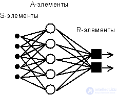
Fig. 4.1. Elementary perceptron of Rosenblatt.

The simplest classical perceptron contains three types of neyrobodobny elements (see. Fig. 4.1), the purpose of which in general corresponds to the neurons of the reflex neural network, discussed in the previous lecture. S-elements form the retina of sensory cells that receive binary signals from the outside world. Next, the signals arrive in a layer of associative or A-elements (to simplify the image, some of the connections from the input S-cells to A-cells are not shown). Only associative elements representing formal neurons perform nonlinear processing of information and have variable link weights. R-elements with fixed weights form the perceptron response signal to the input stimulus.

Rosenblatt called such a neural network three-layer, but according to modern terminology used in this book, the presented network is usually called single-layer , since it has only one layer of neuroprocessor elements. A single-layer perceptron is characterized by a matrix of synaptic connections W from S- to A-elements. Matrix element corresponds to the connection leading from the i-th S-element to the j-th A-element.

In the Cornell Aviation Laboratory, an electrical model of the MARK-1 perceptron was developed, which contained 8 output R-elements and 512 A-elements, which could be combined in various combinations. A series of experiments were carried out on this perceptron to recognize the letters of the alphabet and geometric patterns.

In the works of Rosenblatt, it was concluded that the neural network of the considered architecture will be capable of reproducing any logical function, however, as was shown later by M.Minsky and S. Papert (M.Minsky, S.Papert, 1969), this conclusion was inaccurate. Fundamental unremovable limitations of single-layer perceptrons were identified, and later a multi-layered version of the perceptron, in which there are several layers of processor elements, began to be considered.

From today's standpoint, a single-layer perceptron is more likely to be of historical interest, however, using its example, the basic concepts and simple algorithms for learning neural networks can be studied.

Perceptron training theorem.

Network training consists in adjusting the weights of each neuron. Let there be a set of pairs of vectors (x ^a , y ^a ), a = 1..p, called the training set . We will call a neural network trained in this training sample, if, when each vector x ^{a is} fed to the network inputs, each time, at the outputs, the corresponding vector y ^{a is} obtained

The teaching method proposed by F. Rosenblatt consists in the iterative adjustment of the weights matrix, which successively reduces the error in the output vectors. The algorithm includes several steps:

Step 0.	The initial values ​​of the weights of all neurons rely random.
Step 1.	The network is presented with the input image x a , as a result, the output image is formed
Step 2.	Calculates the error vector made by the network output. A further idea is that the change in the weight coefficient vector in the region of small errors should be proportional to the error at the output, and equal to zero if the error is zero.
Step 3.	The weight vector is modified according to the following formula: . Here - the pace of learning.
Step 4.	Steps 1-3 are repeated for all training vectors. One cycle of sequential presentation of the entire sample is called an epoch . Training ends after several epochs have passed, a) when the iterations converge, i.e. the weight vector ceases to be changed, or b) when the total absolute error over all the vectors becomes less than a certain small value.

The formula used in step 3 takes into account the following circumstances: a) only the components of the weights matrix are modified, corresponding to non-zero values ​​of the inputs; b) the weight increment sign corresponds to the error sign, i.e. a positive error ( d > 0, the output value is less than the required one) leads to increased coupling; c) the learning of each neuron occurs independently of the learning of the rest of the neurons, which corresponds to a biologically important principle of learning locality .

This teaching method was named by F. Rosenblatt “the method of correction with the reverse transmission of the error signal”. Later the name “ d- rule” became more widely known. The presented algorithm belongs to a wide class of learning algorithms with a teacher , since both the input vectors and the required values ​​of the output vectors are known (there is a teacher who is able to evaluate the correctness of the student’s response).

Rosenblatt’s theorem on the convergence of learning by the d- rule says that the perceptron is able to learn any training set that he can imagine . Below we will discuss in more detail the perceptron's ability to present information.

Linear separability and perceptron representability

Each perceptron neuron is a formal threshold element that takes on single values ​​if the total weighted input is greater than a certain threshold value:

Thus, for given values ​​of weights and thresholds, a neuron has a certain value of output activity for each possible input vector. The set of input vectors in which the neuron is active (y = 1) is separated from the set of vectors in which the neuron is passive (y = 0) by a hyperplane , the equation of which is, is:

Consequently, a neuron is able to separate (have a different output) only such two sets of input vectors for which there is a hyperplane that cuts off one set from another. Such sets are called linearly separable . We illustrate this concept with an example.

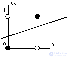
Suppose there is a neuron for which the input vector contains only two Boolean components. defining the plane. On this plane, the possible values ​​of the vectors correspond to the vertices of the unit square. At each vertex, the required value of neuron activity 0 (in Fig. 4.2 - white dot) or 1 (black dot) is determined. It is required to determine whether there is such a set of weights and thresholds of a neuron, at which this neuron can separate points of different colors?

Figure 4.2 presents one of the situations when this can not be done due to the linear inseparability of sets of white and black dots.

Fig. 4.2. White points can not be separated by one straight line from black ones.

The required activity of the neuron for this figure is determined by the table, in which it is not difficult to find out the task of the logical function “exclusive or”.

X 1	X 2	Y
0	0	0
one	0	one
0	one	one
one	one	0

The linear inseparability of a set of arguments that correspond to different values ​​of a function means that the function “exclusive or”, so widely used in logic devices, cannot be represented by a formal neuron. Such modest possibilities of the neuron served as the basis for the criticism of F. Rosenblatt's perceptron direction from M.Minsky and S.Papert.

As the number of arguments increases, the situation is even more catastrophic: the relative number of functions that have the property of linear separability decreases sharply. This means that the class of functions that can be implemented by a perceptron (the so-called class of functions with the perceptron property) can be sharply narrowed. The relevant data is shown in the following table:

Number of variables N	The total number of possible logical functions	Of which are linearly separable functions
one	four	four
2	sixteen	14
3	256	104
four	65536	1882
five	> 1,000,000,000	94572

It can be seen that the single-layer perceptron is extremely limited in its ability to accurately represent in advance the specified logical function. It should be noted that later, in the early 70s, this restriction was overcome by introducing several layers of neurons, but the critical attitude to the classical perceptron strongly froze the general range of interest and research in the field of artificial neural networks.

In conclusion, let us dwell on the problems that remained open after the works of F. Rosenblatt. Some of them were subsequently solved (and will be partially considered in the next lectures), some were left without a complete theoretical solution.

1. Practical verification of the condition of linear separability of sets. Rosenblatt's theorem guarantees successful learning only for perceptron-representable functions, but says nothing about how to practically detect this property before learning.
2. How many steps are required for iterative learning? In other words, prolonged learning can be both a consequence of the non-representability of a function (and in this case it will never end), or just a feature of the algorithm.
3. How does the sequence of presentation of images during the training era affect learning?
4. Does the d- rule have any advantages over simple enumeration of scales, i.e. Is it a constructive fast learning algorithm?
5. What will be the quality of training if the training sample does not contain all possible pairs of vectors? What will be the perceptron responses to the new vectors?

The last question involves deep layers of computational neuroscience regarding the capabilities of artificial systems to generalize limited individual experience into a wider class of situations for which the response was not previously communicated to the neural network. The situation when the system has to work with new images is typical, since the number of all possible examples grows exponentially quickly with an increase in the number of variables, and therefore, in practice, the individual experience of the network is always fundamentally not complete.

The possibilities of generalization in neural networks will be discussed in more detail in the next lecture.