Lecture
The Mamdani algorithm is used for multi-criteria evaluation of objects based on a set of criteria [15]. The input data for the algorithm are the description and values of fuzzy variables, the rules of inference. The result of the algorithm are clear values of the output variables.
At the first stage, the set of criteria k 1 is determined , k 2 , ..., k v for evaluating objects, they are assigned fuzzy variables.
Fuzzy variables represent a triplet <a, X, A >, where a is the variable name, X is the domain of a, A is a fuzzy set on X , which can be characterized by a set of membership functions m A (x). The sets X and A are determined by a specific criterion. For example, if the “location of the firm” acts as a criterion, then the fuzzy variable of the same name will correspond to it, the set of values of which can be described by the triple “convenient”, “not very convenient”, “inconvenient”. Each value will have its own membership function.
The rules are constructions of the form.
“If <complex condition>, then <list of outputs>”, where
<complex condition>: - or (<list of conditions>) |
and (<list of conditions>) |
<condition>
<list of conditions>: - (<condition>) [<list of conditions>]
<condition>: - <name of input fuzzy variable>
<value of input fuzzy variable>
<output list>: - (<output value>) [<output list>]
<output value>: - <output fuzzy variable name>
<value of output fuzzy variable>
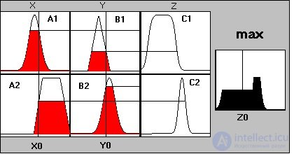
Consider the work of the Mamdani algorithm on an example (Fig.4.5). Let the knowledge base consists of two rules:
P1: if x is A1 and y is B1 , then z is C1 ,
P2: if x is A2 and y is B 2 , then z is C2 ,
where x and y are the names of the input variables, z is the name of the output variable, A 1, A 2, B 1, B 2, C 1, C 2 are some specified membership functions, and the clear value of z 0 must be determined on the basis of the information provided. and clear values x 0 and y 0 .

Fig. 4.5. The main stages of the Mamdani algorithm
The algorithm consists of 4 stages:
1. Introducing fuzziness: find the degrees of truth for the premises of each rule: A1 ( x 0 ), A2 ( x 0 ), B1 ( y 0 ), B2 ( y 0 ). For example, A1 ( x 0 ) is the value of the membership function A1 for the variable x at the point x 0 .
2. Fuzzy conclusion: there are “cut-off” levels for the premises of each of the rules (the operation min is used for the logical operation “and”, the operation max is used for the logical operation “or”).
a 1 = A 1 ( x 0 ) B 1 ( y 0 )
a 2 = A 2 ( x 0 ) B 2 ( y 0 )
Then the truncated membership functions for the output variable are found.
C ' 1 = ( a 1 Ù C1 (z))
C ' 2 = ( a 2 Ù C2 (z))
3. Composition: using the max operation, the found truncated functions are combined, which results in the final membership function for the output variable.
μ S ( z ) = C ( z ) = C ' 1 Ú C' 2 = ( a 1 C 1 ( z )) Ú ( a 2 C 2 ( z )) =
= (A1 (x 0 ) Ù B1 (y 0 ) Ù C1 (z)) (A2 (x 0 ) Ù B2 (y 0 ) C2 (z))
4. Defusification: there is a clear value for the output variable. z 0 (for example, by the centroid method (as the center of gravity for the μ S (z) curve):
 - for the discrete version.
An example of building a rating of computer companies based on the Mamdani method
The criteria for the evaluation of objects in this case are the "quality of customer service" and "location of the company." Both criteria are measured on a five-point scale, that is, the expert can choose any integer in the range from 0 to 5 as the value of the criterion. We put the criteria in accordance with fuzzy variables (Table 4.10).
Table 4.10
Fuzzy variable parameters | The name of a fuzzy variable a | |
"Quality of customer service" (KO) | "The location of the company" (MF) | |
Scope X | [0,5] | [0,5] |
Fuzzy variable values | “Excellent”, “acceptable”, “bad” | "Comfortable", "not very comfortable", "uncomfortable" |
Membership function
|  |  |
The output variable will be “object rating” (Table 4.11).
Table 4.11
The name of a fuzzy variable a | "Rating" |
Scope X | [0,100] |
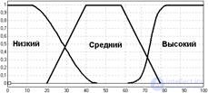
Fuzzy variable values | "Low", "medium", "high" |
Membership function |  |
For ease of calculation, let the inference rule system consist of 3 rules.
P1: If KO is excellent (A1) and MF is uncomfortable (B1), then the rating is average (C1).
P2: If KO is acceptable (A2) and MF is not very convenient (B2), then the rating is low (C2).
P3: If KO is bad (A3) and MF is convenient (B3), then the rating is low (C3).
Baseline data will be presented in the form of table 4.12
Table 4.12
Company number | Quality of service, points | Location, points |
one | four | one |
2 | 3 | 3 |
3 | one | four |
Consider the main stages of the algorithm.
Stage 1. Introduction of fuzziness
Find the degrees of truth for the premises of each rule.
Table 4.13
Company number | P1 | P2 | A3 |
one | A1 (4) = 0.5, B1 (1) = 0.35 | A2 (4) = 0, B2 (1) = 0 | A3 (4) = 0, B3 (1) = 0 |
2 | A1 (3) = 0, B1 (3) = 0 | A2 (3) = 1, B2 (3) = 0.65 | A3 (3) = 0, B3 (3) = 0 |
3 | A1 (1) = 0, B1 (4) = 0 | A2 (1) = 0, B2 (4) = 0 | A3 (1) = 0.5, B3 (4) = 0.3 |
Stage 2. Fuzzy output
Find the clipping levels for the premises of each of the rules.
Table 4.14
Company number | P1 | P2 | A3 |
one | a 1 = min (0.5,0.3 5 ) = 0.3 5 | a 2 = min (0,0) = 0 | a 3 = min (0,0) = 0 |
2 | a 1 = min (0,0) = 0 | a 2 = min (1,0.65) = 0.65 | a 3 = min (0,0) = 0 |
3 | a 1 = min (0,0) = 0 | a 2 = min (0,0) = 0 | a 3 = min (0.5,0.3) = 0.3 |
Find the truncated membership functions for the output variable.
Table 4.15
Company number | P1 | P2 | A3 |
one | C ' 1 = a 1 Ù C 1 ( 0.3 5) | C ' 2 = a 2 Ù C2 (0) | C ' 3 = a 3 Ù C3 (0) |
2 | C ' 1 = a 1 Ù C 1 ( 0 ) | C ' 2 = a 2 Ù C (0.65) | C ' 3 = a 3 Ù C3 (0) |
3 | C ' 1 = a 1 Ù C 1 ( 0 ) | C ' 2 = a 2 Ù C2 (0) | C ' 3 = a 3 Ù C3 (0.3) |
Stage 3 and 4. Composition and defuzzification
Table 4.16
Company number | μ S ( z ) = C ( z ) = C ' 1 Ú C' 2 C ' 3 | μ S (z) | z i | Rating |
one | max (0.35,0,0) = 0.3 5 |  | 50 | one |
2 | max (0,0.65 , 0 ) = 0.65 |  | 16.7 | 3 |
3 | max (0, 0, 0.3) = 0.3 |  | 18.62 | 2 |
Thus, as a result of the algorithm, we have a set of clear values for the output variable “rating” in our chosen scale of measurement of the variable values: z 1 , z 2 , ..., z m , where m is the number of firms. Sorting the obtained values in descending order, we obtain the rating of firms P.
Comments
To leave a comment
Decision theory
Terms: Decision theory