
Lecture
In the design of pressure pipelines, the main problem is either determining the flow capacity (discharge), or the head loss at a given section as well as over the entire length, or the diameter
of the pipeline for a given discharge and head loss. In practice, pipelines are divided into short and long ones. The first group includes all pipelines in which local head losses exceed 5…10% of the head loss along the length. When calculating such pipelines, head losses in local resistances must be taken into account. These include, for example, oil lines of volumetric drives.
The second group includes pipelines in which local losses are less than 5…10% of the head loss along the length. Their calculation is carried out without accounting for local losses. Such pipelines include, for example, trunk water mains and oil pipelines.
Considering the hydraulic layout of long pipelines, they can also be divided into simple and complex ones. Simple pipelines are pipelines of the same or different cross-sections connected in series, with no branches whatsoever. Complex pipelines include systems of pipes with one or several branches, parallel lines, etc. So-called looped (ring) pipelines are also classified as complex.
Liquid moves through a pipeline because its energy at the beginning of the pipeline is greater than at the end. This drop in energy level can be created in several ways: by the operation of a pump, by a difference in liquid levels, or by gas pressure.
Let us consider a simple pipeline of constant cross-section, arbitrarily located in space (Fig. 6.1), having overall length and diameter d, and also containing a number of local resistances (a valve, a filter, and a check valve). At the initial section of the pipeline 1-1, the geometric elevation equals z1 and the gauge pressure P1, while at the final section 2-2 – z2 and P2, respectively. Due to the constant pipe diameter, the flow velocity at these sections is the same and equals .
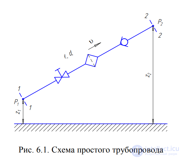
Fig. 6.1. Diagram of a simple pipeline
Let us write the Bernoulli equation for sections 1-1 and 2-2. Since the velocity is the same in both sections and 1 = 2, the velocity head can be disregarded. This gives
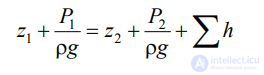
or
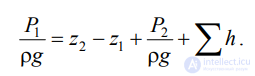 . (6.1)
Let us call the piezometric head appearing on the left-hand side of the equation the required head Hreq. If, on the other hand, this piezometric head is given, it is called the available head Havail. Such a head consists of the geometric elevation Δz = z2 – z1, through which the liquid rises, the piezometric head at the end of the pipeline, and the sum of all head losses in the pipeline.
Let us call the sum of the first two terms the static head, which we can represent as a certain equivalent geometric
elevation
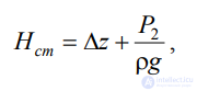
,
and the last term h – as a power function of the discharge
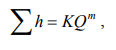 ,
,
then
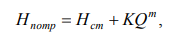 , (6.2)
where K – is a quantity called the pipeline resistance;
Q – is the liquid discharge;
m – is an exponent that takes different values depending on the flow regime.
For laminar flow, when local resistances are replaced by equivalent lengths, the pipeline resistance equals
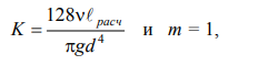 , (6.3)
where 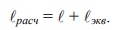 .
.
Numerical values of the equivalent lengths eq for various local resistances are usually found experimentally.
For turbulent flow, using the Weisbach-Darcy formula (4.9) and expressing the velocity in it in terms of the discharge, we obtain
 (6.4)
(6.4)
Formula (6.2), supplemented by expressions (6.3) and (6.4), is the fundamental formula for calculating simple pipelines. From it one can plot the required-head curve as a function of discharge. The greater the discharge Q that must be provided in the pipeline, the greater the required head Hreq must be. For laminar flow, this curve is represented by a straight line (Fig. 6.2, a); for turbulent flow – by a parabola with an exponent of two (Fig. 6.2, b).
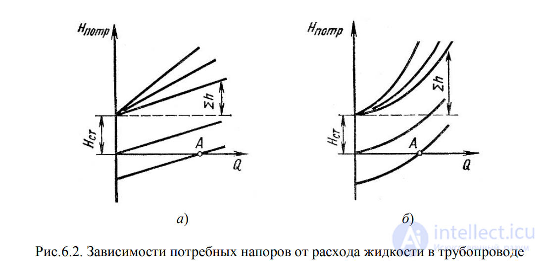
Fig. 6.2. Dependence of the required head on the liquid discharge in a pipeline
The steepness of the required-head curves depends on the pipeline resistance K and increases with increasing pipeline length and decreasing diameter, as well as with increasing local hydraulic resistances.
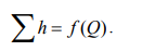
The static head Hst is positive when the liquid moves upward or into a cavity with higher pressure, and negative when the liquid descends or moves into a cavity with lower pressure. The point where the required-head curve intersects the abscissa axis (point A) determines the discharge for gravity flow of the liquid. In this case the required head equals zero. Sometimes, instead of required-head curves, it is more convenient to use pipeline characteristics. The characteristic of a pipeline is the relationship between the total head (or pressure) loss in the pipeline and the discharge:
 .
.
Simple pipelines can be connected to one another, and such a connection can be either series or parallel. Series connection. Let us take several pipes of different lengths, different diameters, and containing different local resistances, and
connect them in series (Fig. 6.3, a).
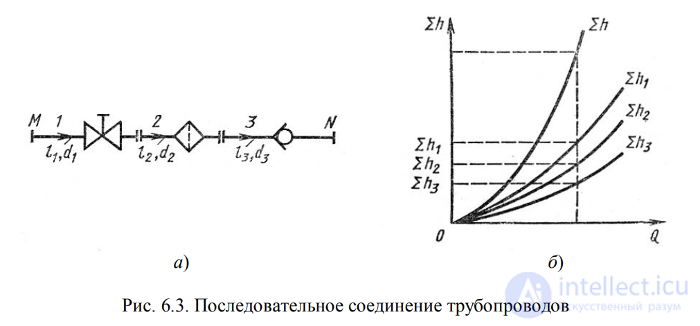
Fig. 6.3. Series connection of pipelines
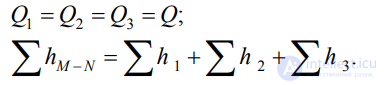
When liquid is delivered through such a composite pipeline from point M to point N, the discharge Q in all the series-connected pipes 1, 2, and 3 will be the same, while the total head loss between points
M and N equals the sum of the head losses in all the series-connected pipes. Thus, for a series connection we have the following basic equations:
(6.5)
These equations determine the rules for constructing the characteristic of a series connection of pipes (Fig. 6.3, b). If the characteristics of each pipeline are known, then the characteristic of the entire series connection M-N can be constructed from them.
To do this, the ordinates of all three curves must be added.
Parallel connection. Such a connection is shown in Fig. 6.4, a. Pipelines 1, 2, and 3 are arranged horizontally.
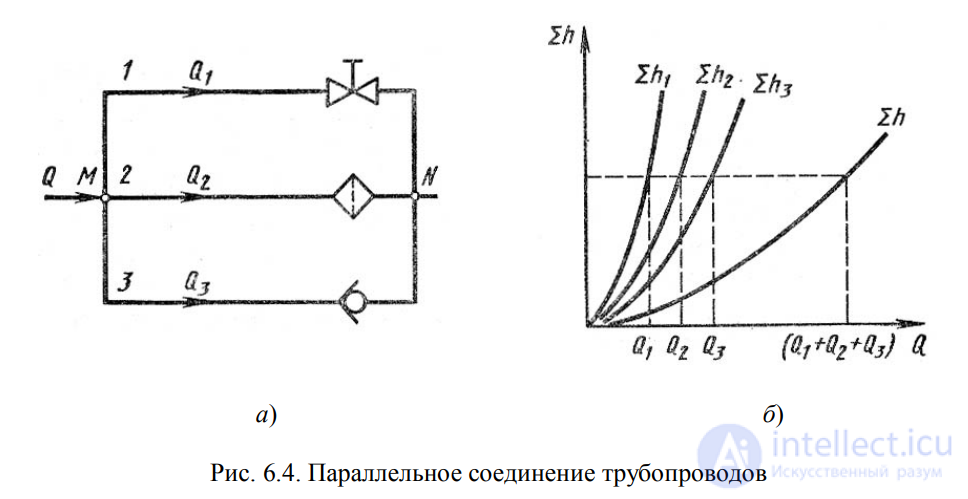
Fig. 6.4. Parallel connection of pipelines
Let us denote the total heads at points M and N as HM and HN respectively, the discharge in the main line (i.e., before the branching and after the merging) – by Q, and in the parallel pipelines by Q1, Q2, and Q3; the total losses in these pipelines by  .
.
Obviously, the liquid discharge in the main line is
Q = Q1 + Q2+ Q3 (6.6)
Let us express the head loss in each of the pipelines in terms of the total heads at points M and N:

From this we conclude that
 (6.7)
(6.7)
i.e., the head losses in the parallel pipelines are equal to one another. They can be expressed in general form through the corresponding discharges as follows

,
where K and m – are determined depending on the flow regime by formulas (6.3) and (6.4).
From equations (6.6) and (6.7) the following rule follows: to construct the characteristic of a parallel connection of several
pipelines, one must add the abscissas (discharges) of the characteristics of these pipelines at equal ordinates  . An example of such a construction is given in Fig. 6.3, b.
Branched connection. A branched connection is a set of several simple pipelines having one common section – the point of branching (or merging) of the pipes.
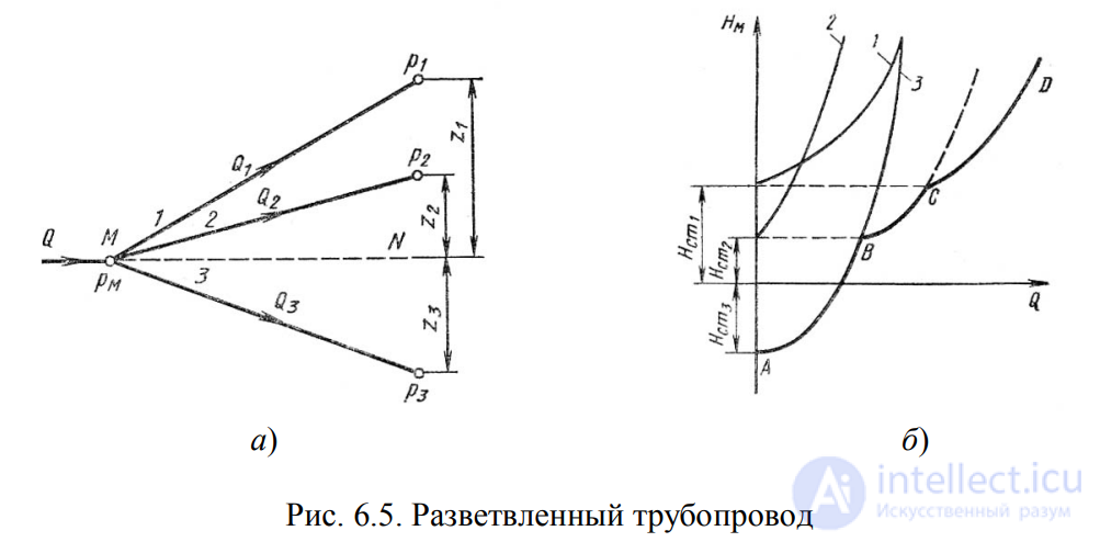
Fig. 6.5. Branched pipeline
Suppose the main pipeline has a branching at section M-M, from which, for example, three pipes 1, 2, and 3 of different diameters branch off, containing different local resistances (Fig. 6.5, a). The geometric elevations z1, z1, and z1 of the end sections and the pressures P1, P2, and P3 at them will also be different.
As with parallel pipelines, the total discharge in the main pipeline will equal the sum of the discharges in each pipeline:
Q = Q1 + Q2 + Q3 . (6.8)
Writing the Bernoulli equation for section M-M and the end section, for example, of the first pipeline, we obtain (neglecting the difference in velocity heads)
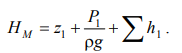
Denoting the sum of the first two terms by Hst and expressing the third term in terms of the discharge (as was done in section 6.1), we obtain
 . (6.9)
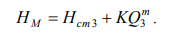
Similarly, for the other two pipelines we can write
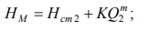 ; (6.10)
 . (6.11)
Thus, we obtain a system of four equations with four unknowns: Q1, Q2, Q3, and HM.
Constructing the required-head curve for a branched pipeline is done by adding the required-head curves for the branches according to the rule for adding the characteristics of parallel pipelines (Fig. 6.5, b) – by adding the abscissas (Q) at equal ordinates (HM). The required-head curves for the branches are marked with the numbers 1, 2, and 3, and the total required-head curve for the entire branched system is denoted by the letters ABCD. From the graph it can be seen that the condition for delivering liquid to all branches is the inequality HM > Hst1.
A complex pipeline in the general case is made up of simple pipelines connected in series and in parallel (Fig. 6.6, a) or with branches (Fig. 6.6, b).
a) b)
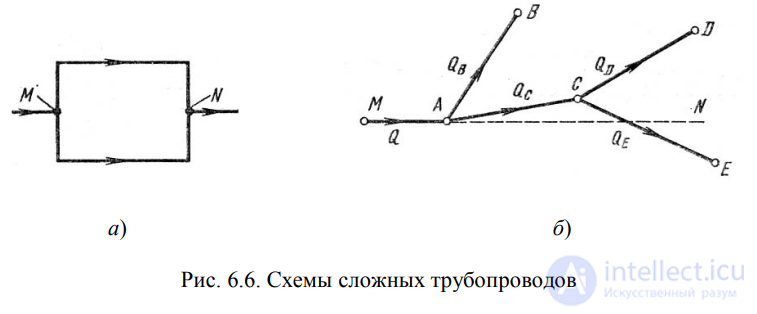
Fig. 6.6. Diagrams of complex pipelines
Let us consider an open-type complex pipeline (Fig. 6.6, b). The trunk pipeline branches at points A and C. Liquid is delivered to points (sections) B, D, and E with discharges QB, QD, and QE. Suppose the dimensions of the trunk line and all branches (simple pipelines) are known, all local resistances are given, as well as the geometric elevations of the end points, measured from the plane M-N, and the gauge pressures at the end points PB, PD, and PE. In this
case there can be
For this case two types of problems are possible:
Problem 1. Given the discharge Q in the main trunk line MA. It is required to determine the discharges QB, QD, QE, as well as the required head at point M.
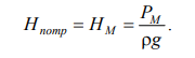
Problem 2. Given the head at point M. Determine the discharge in the trunk line Q and the discharges in each branch.
Both problems are solved on the basis of the same system of equations, the number of which is one more than the number of end branches, namely:
the discharge equation:

the equation of equality of required heads for branches CD and CE

the equation of equality of required heads for branch AB and complex pipeline ACED

the expression for the required head at point M

Calculation of complex pipelines is often performed by the graphoanalytical method, i.e., using required-head curves and pipeline characteristics. The required-head curve for a complex pipeline should be constructed as follows:
1) the complex pipeline is broken down into a number of simple ones;
2) required-head curves are constructed for each of the simple pipelines;
3) the required-head curves for the branches (and parallel lines, if any) are added according to the rule for adding the characteristics of parallel pipelines;
4) the resulting curve is added to the characteristic of the series-connected pipeline according to the corresponding rule (see section 6.2).
Thus, in the calculation one proceeds from the end points of the pipeline to the starting point, i.e., against the flow of the liquid.
Complex looped (ring) pipeline. This is a system of adjacent closed loops, with liquid withdrawal at nodal points or with continuous liquid distribution along individual sections (Fig. 6.7).
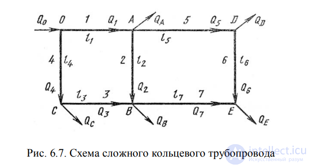
Fig. 6.7. Diagram of a complex looped pipeline
Problems for such pipelines are solved by an analogous method using electrical analogies (Kirchhoff's law). This is based on two mandatory conditions. The first condition – the discharge balance, i.e., equality of inflow and outflow of liquid at each nodal point. The second condition – the head balance, i.e., the algebraic sum of the head losses for each loop (circuit) is equal to zero when calculated in the clockwise or counterclockwise direction.
For the calculation of such pipelines, the following is a typical problem. Given the maximum head at the starting point, i.e., at point 0, the minimum head at the most distant point E, the discharges at all six nodes, and the lengths of the seven sections. It is required to determine the diameters of the pipelines on all sections.
As already noted above, the drop in energy level, due to which the liquid flows through the pipeline, can be created by the operation of a pump, which is widely used in mechanical engineering. Let us consider the joint operation of a pipeline with a pump and the principle of calculating a pipeline with pump delivery of liquid.
A pipeline with pump delivery of liquid can be of the open type, i.e., through which liquid is pumped from one reservoir to another (Fig. 6.8, a), or of the closed (looped) type, in which the same quantity of liquid circulates (Fig. 6.8, b).
a) b)
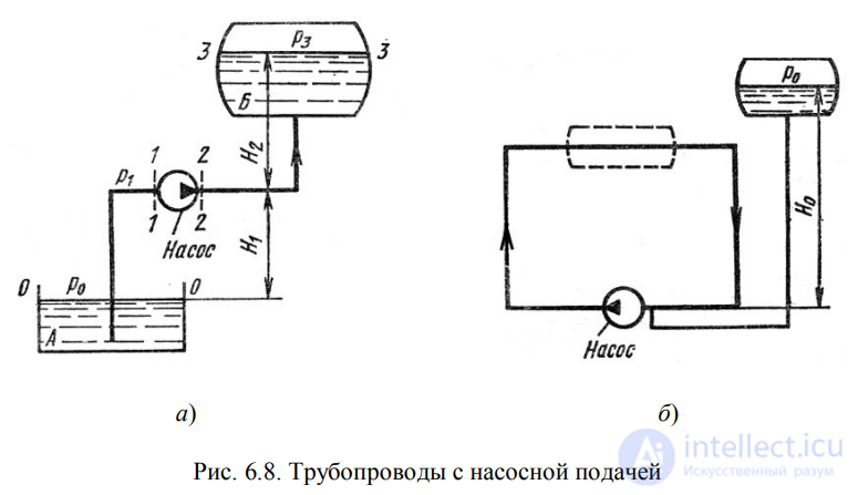
Fig. 6.8. Pipelines with pump delivery
Let us consider a pipeline through which liquid is pumped from a lower reservoir at pressure P0 to another reservoir at pressure P3 (Fig. 6.8, a). The elevation of the pump axis H1 is called the geometric suction lift, and the pipeline through which the liquid enters the pump is called the suction pipeline or suction line. The elevation of the end section of the pipeline H2 is called the geometric discharge head, and the pipeline through which the liquid moves from the pump is called the discharge pipeline or discharge line. Let us write the Bernoulli equation for the flow of the working liquid in the suction pipeline, i.e., for sections 0-0 and 1-1 (taking α=1):
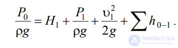 . (6.12)
This equation is the fundamental one for calculating suction pipelines.
Now let us consider the discharge pipeline, for which we write the Bernoulli equation, i.e., for sections 2-2 and 3-3:
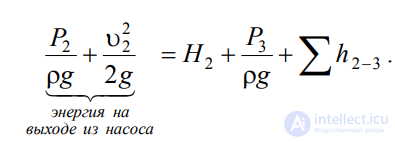 . (6.13)
The left-hand side of equation (6.13) represents the energy of the liquid at the pump outlet. And the energy of the liquid at the pump inlet can similarly be expressed from equation (6.12):
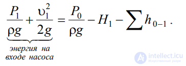 . (6.14)
In this way, one can calculate the increase in energy of the liquid passing through the pump. This energy is imparted to the liquid by the pump and is therefore usually denoted Hpump.
To find the head Hpump created by the pump, let us subtract equation (6.14) from equation (6.13):

or
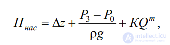
, (6.15)
where Δz - is the total geometric lift height of the liquid, Δz = H1 + H2;
KQ m– is the sum of the hydraulic losses,
P3 and P0 – are the pressures in the upper and lower reservoirs, respectively.
If, to the actual level difference Δz, we add the difference of the piezometric heads (P3 - P0)/(ρg), then we can consider an increased level difference
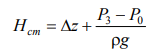
and formula (6.15) can be rewritten as
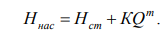 . (6.15')
If we compare the resulting expression (6.15') with formula (6.2) for the required head, we can conclude that
Hpump = Hreq . (6.16)
From this follows the rule for stable operation of a pump: under steady-state liquid flow in a pipeline, the pump develops a head equal to the required head.
Based on equality (6.16), a method for calculating pipelines with pump delivery is based on the joint plotting, on the same
scale and on the same graph, of two curves: the required-head curve Hreq = f1(Q) and the pump characteristic Hpump = f2(Q), and finding their point of intersection (Fig. 6.9).
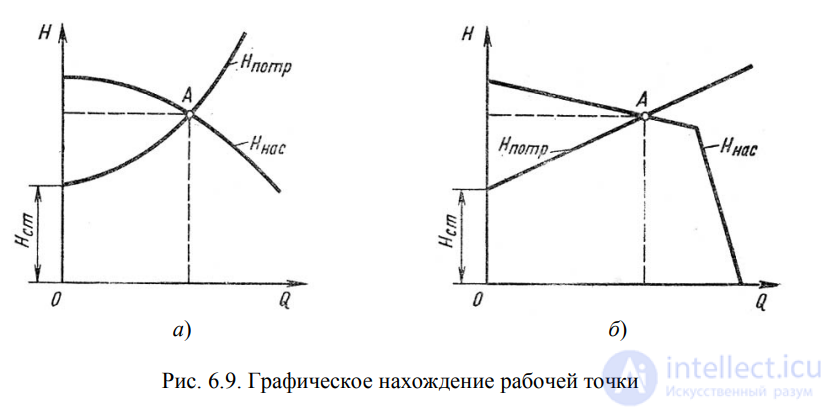
Fig. 6.9. Graphical determination of the operating point The pump characteristic is defined as the relationship between the head developed by the pump and its flow rate (liquid discharge) at a constant pump shaft rotational speed. Fig. 6.9 shows two versions of the graph: a – for turbulent flow; b – for laminar flow. The point of intersection of the required-head curve with the pump characteristic is called the operating point. To obtain a different operating point, it is necessary to change the opening of the control valve (changing the pipeline characteristic) or to change the pump shaft rotational speed.
Water hammer is a sharp rise in pressure that occurs in a pressure pipeline upon sudden deceleration of the working-liquid flow. This process is very fast and is characterized by alternating sharp increases and decreases in pressure, associated with elastic deformations of the liquid and the pipeline walls. Water hammer most often occurs upon sudden opening or closing of a valve or other flow-controlled device.
Suppose that at the end of a pipe, through which liquid moves at a velocity
ν0, instantaneous closure of the valve occurs (Fig. 6.10, a).
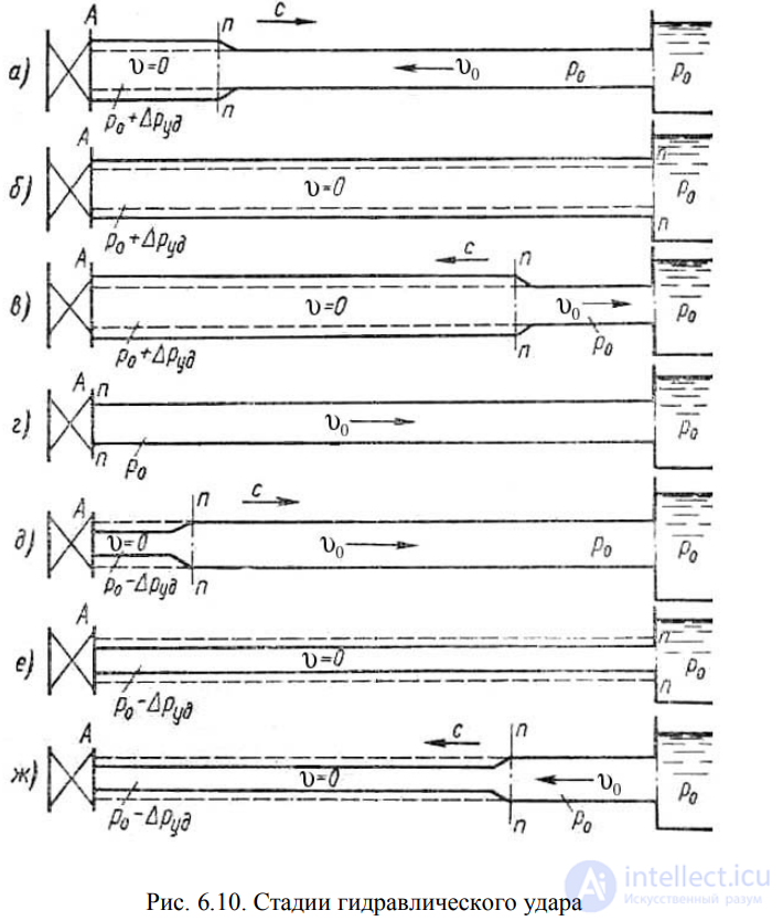
Fig. 6.10. Stages of water hammer
In this case, the velocity of the particles striking the valve will be brought to zero,
and their kinetic energy will be converted into the work of deformation of the pipe walls and
the liquid. The pipe walls stretch, while the liquid is compressed in
accordance with an increase in pressure by an amount Pshock, which
is called the shock pressure. The region (section n – n) in which the pressure increase occurs is called the pressure wave (shock wave).
The shock wave propagates to the right at a velocity c, called the shock wave velocity.
When the shock wave reaches the reservoir, the liquid becomes
stopped and compressed throughout the entire pipe, and the pipe walls – stretched.
The shock pressure rise spreads over the entire length of the pipe
(Fig. 6.10, b).
Then, under the action of the pressure drop Δ Pshock, particles of liquid
rush from the pipe into the reservoir, and this flow begins at the section
directly adjacent to the reservoir. Now the section n-n
moves back toward the valve at the same velocity c, leaving behind it
an equalized pressure P0 (Fig. 6.10, c).
The liquid and the pipe walls are assumed to be elastic, so they
return to their previous state, corresponding to pressure P0.
The work of deformation is fully converted into kinetic energy, and
the liquid in the pipe acquires its original velocity 0, but
now directed in the opposite direction.
With this velocity, the entire volume of liquid tends to separate from the
valve, and as a result a negative shock wave arises, at a pressure
P0 - Δ Pshock, which travels from the valve toward the reservoir at velocity c,
leaving behind it compressed pipe walls and expanded liquid,
which is due to the pressure drop (Fig. 6.10, d). The kinetic energy of the
liquid again converts into the work of deformation, but of the opposite
sign.
The state of the pipe at the moment the negative shock wave arrives at the
reservoir is shown in Fig. 6.10, e. As in the case
shown in Fig. 6.10, b, it is not an equilibrium state. In
Fig. 6.10, f, the process of pressure equalization in the pipe and
reservoir is shown, accompanied by the onset of liquid motion at
velocity 0.
Obviously, as soon as the shock wave reflected from the reservoir,
at pressure Pshock, reaches the valve, a situation arises that has already occurred
at the moment the valve was closed. The entire water-hammer cycle
repeats.
The course of water hammer over time is illustrated by the
diagram shown in Fig. 6.11, a and b.
The dashed lines show the theoretical variation of pressure
at the valve at point A, while the solid line shows the actual pattern of pressure
variation over time (Fig. 6.11, a). Here, the damping of pressure
oscillations occurs due to the loss of liquid energy overcoming
friction forces and the dissipation of energy into the reservoir.
If the pressure P0 is small (P0 < Pshock), the pattern of variation of the
pressure amplitude turns out to be somewhat different, approximately as
shown in Fig. 6.11, b.
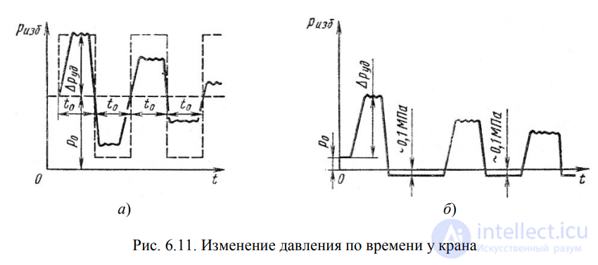
Fig. 6.11. Variation of pressure over time at the valve
The pressure rise during water hammer can be determined
by the formula
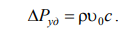 . (6.17)
This expression is known as the Zhukovsky formula. In it, the
propagation velocity of the shock wave c is determined by the formula:
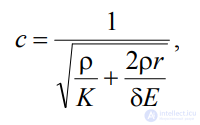 , (6.18)
where r – is the pipeline radius;
E – is the modulus of elasticity of the pipe material;
δ – is the pipeline wall thickness;
K – is the bulk modulus of elasticity (see section 1.3)
If we assume that the pipe has absolutely rigid walls, i.e.,
E =  , then the shock wave velocity is determined from the expression
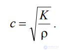 . (6.19)
For water this velocity equals 1435 m/s, for gasoline 1116 m/s, for
oil 1200 - 1400 m/s.
When designing pressure pipelines, it should be taken into account that their flow capacity decreases during operation (for example, for water-supply pipes, by up to 50% or even lower). Due to corrosion and the formation of deposits in the pipes (incrustation), the pipe roughness increases. This can be estimated by the formula:
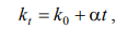
where k0 – is the absolute roughness for new pipes, (mm),
kt – is the roughness after t years of operation,
α – is a coefficient characterizing the rate of increase of roughness (mm/year).
Table 6.1
Value of the coefficient α depending on the physicochemical properties of the transported water
| Corrosive action | Characteristics of natural waters | α, mm/year |
|---|---|---|
| Weak | Weakly mineralized non-corrosive waters with a low content of organic substances and dissolved iron. | 0.005–0.055 (average 0.025) |
| Moderate | Weakly mineralized corrosive waters containing organic substances and dissolved iron in an amount of 3 mg/L. | 0.035–0.18 (average 0.07) |
| Significant | Highly corrosive waters with an iron content of more than 30 mg/L, but with a low chloride content. | 0.18–0.40 (average 0.20) |
| Strong | Chloride and sulfate content greater than 500–700 mg/L, as well as untreated waters with a high content of organic substances. | 0.40–0.60 (average 0.51) |
| Very strong | Water with significant carbonate and low permanent hardness, with a total dissolved solids content greater than 2000 mg/L, highly mineralized and corrosive. | from 0.6 to 1 or more |

Comments