
Lecture
Energy losses (a decrease in hydraulic head) can
be observed in moving fluid not only over comparatively long
sections, but also over short ones. In some cases the head
losses are distributed (sometimes uniformly) along the length of the pipeline – these are
linear (friction) losses; in other cases they are concentrated over very short
sections, whose length can be neglected – at the so-called
local hydraulic resistances: valves, various
bends, contractions, expansions, etc., in short, wherever the flow
undergoes deformation. In all cases, the source of the losses is
the viscosity of the fluid.
It should be noted that head losses, both along the length and at local
hydraulic resistances, depend substantially on the so-
called flow regime of the fluid.
When observing the motion of fluid in pipes and channels, it can
be noticed that in one case the fluid maintains a certain order
of its particles, while in others it moves in a disorderly manner. However,
exhaustive experiments on this question were carried out by Reynolds in
1883. Fig. 4.1 shows an apparatus similar to the one on which
Reynolds conducted his experiments.
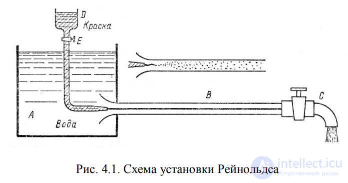
Fig. 4.1. Diagram of Reynolds' apparatus
The apparatus consists of a reservoir A with water, from which a
glass tube B with a valve C at the end extends, and a vessel D with an aqueous solution
of dye, which can be introduced through a tube as a thin stream into the
interior of the glass tube B.
First case of fluid motion. If valve
C is opened slightly, allowing water to flow through the tube at a low velocity, and
dye is then let into the water flow by means of valve E, we will see that
the dye introduced into the tube does not mix with the water flow.
The dye streak remains clearly visible along the entire length of the glass tube,
which indicates the layered (laminar) nature of the flow and the absence of
mixing. Moreover, if a piezometer or a
Pitot tube is connected to the pipe, they will show that pressure and velocity remain
constant over time. This flow regime is called laminar.
Second case of fluid motion. As the
water flow velocity in the pipe is gradually increased by opening valve C, the flow
pattern at first does not change, but then, at a certain flow velocity,
a rapid change occurs in it. The dye streak, upon leaving the tube,
begins to oscillate, then becomes blurred and mixes with the water
flow, and vortex formation and rotational
motion of the fluid become noticeable. The piezometer and Pitot tube will then show
continuous pulsations of pressure and velocity in the water flow. Such a flow
is called turbulent (Fig. 4.1, top).
If the flow velocity is reduced, the laminar
flow is restored.
Thus, laminar flow is defined as layered flow without mixing
of fluid particles and without pulsation of velocity and pressure. In laminar
flow of a fluid in a straight pipe of constant cross-section, all streamlines
are directed parallel to the pipe axis, and there are no transverse
displacements of fluid particles.
Turbulent flow is defined as flow accompanied by
intensive mixing of the fluid with pulsations of velocities and
pressures. Along with the main longitudinal motion of the fluid,
transverse displacements and rotational motions
of individual fluid volumes are observed. The transition from the laminar regime to the
turbulent one occurs at a certain fluid
flow velocity. This velocity is called the critical velocity, cr.
The value of this velocity is directly proportional to the kinematic
viscosity of the fluid and inversely proportional to the pipe diameter.
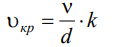 (4.1)
(4.1)
where – is the kinematic viscosity;
k – a dimensionless coefficient;
d – the internal diameter of the pipe.
The dimensionless coefficient k in this formula is the same
for all liquids and gases, and for any pipe diameters. This
coefficient is called the critical Reynolds number Recr and
is defined as follows:
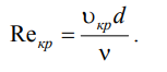 (4.2)
(4.2)
As experiments show, for pipes of circular cross-section Recr ≈ 2300.
Thus, the Reynolds similarity criterion makes it possible to judge the
flow regime of a fluid in a pipe. At Re < Recr the flow is
laminar, and at Re > Recr the flow is turbulent. More precisely,
fully developed turbulent flow in pipes is established
only at Re > 4000, while at Re = 2300…4000 there is a transitional,
critical region.
The flow regime of a fluid directly affects the degree of
hydraulic resistance of pipelines.
In some cases, when a fluid moves in closed channels,
a phenomenon occurs that is related to a change in the state of aggregation of the
fluid, i.e., its conversion into vapor with the release from the fluid
of gases dissolved in it.
This phenomenon can be clearly demonstrated on a simple
device consisting of a pipe, in a separate section of which a
transparent Venturi tube is installed (Fig. 4.2). Water under pressure
moves from section 1-1 through section 2-2 to section 3-3. As can be seen from
the figure, section 2-2 has a smaller diameter. The velocity of the fluid flow
in the pipe can be varied, for example, by a valve
installed after section 3-3.
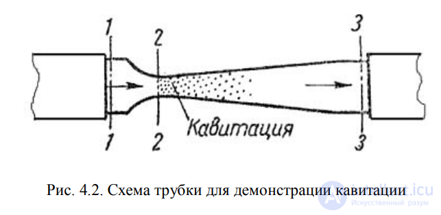
Fig. 4.2. Diagram of a tube for demonstrating cavitation
At low velocity, no visible changes occur in the motion of the
fluid. As the fluid flow velocity increases, a distinct zone with
gas bubble formation appears in the narrow section 2-2 of the Venturi tube.
A region of local boiling forms, i.e.,
vapor forms with the release of gas dissolved in the water.
Further, as the fluid approaches section 3-3, this phenomenon disappears.
This phenomenon is caused by the following. It is known that as a
liquid or gaseous medium moves, the pressure in it drops. Moreover, the higher the
velocity of the medium's motion, the lower the pressure in it. Therefore, as
fluid flows through the local constriction 2-2, in accordance with the continuity equation
of flow (3.4), the velocity increases with a simultaneous drop in
pressure at that location. If the absolute pressure at that point reaches
a value equal to the saturated vapor pressure of the fluid at the given
temperature, or a value equal to the pressure at which
the release of dissolved gases from it begins, then at that point in the flow
intensive vapor formation (boiling) and gas release are observed.
This phenomenon is called cavitation.
As the fluid continues to move toward section 3-3, the bubbles
disappear, i.e., a sharp decrease in their size occurs. At the moment
when a bubble disappears (collapses), at the point of its collapse
a sharp increase in pressure occurs, which is transmitted to neighboring
volumes of fluid and, through them, to the walls of the pipeline. Thus, from
such numerous local pressure surges (water hammers),
vibration arises.
Thus, cavitation is a local disruption of the continuity of the
flow with the formation of vapor and gas bubbles (cavities),
caused by a local drop in pressure in the flow.
In ordinary cases cavitation is an undesirable phenomenon, and
it should not be allowed to occur in pipelines and other elements of hydraulic systems.
Cavitation occurs in cocks, valves, gate valves, nozzles, etc.
Cavitation can occur in hydraulic machines (pumps and
hydraulic turbines), reducing their efficiency, and
prolonged exposure to cavitation causes destruction of parts
subject to vibration. In addition, the walls of pipelines are destroyed,
and their throughput capacity decreases due to the reduction of the effective
cross-section of the pipe.
As studies show, in laminar fluid flow in a
circular pipe, the maximum velocity is on the pipe axis. At the walls
of the pipe, the velocity is zero, because fluid particles cover the
inner surface of the pipe with a thin stationary layer. From the
pipe walls to its axis, the velocity increases smoothly. The graph of the
velocity distribution over the cross-section of the flow is a
paraboloid of revolution, and the cross-section of the paraboloid by an axial plane is
a quadratic parabola (Fig. 4.3).
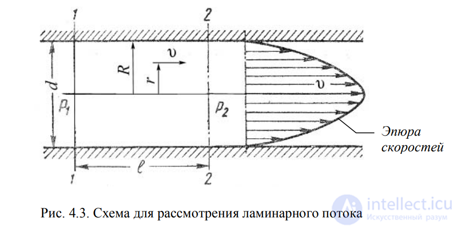
Fig. 4.3. Diagram for considering laminar flow
The equation relating the variables and r has the following
form:
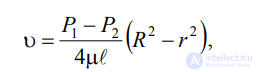 , (4.3)
where P1 and P2 – are the pressures in sections 1 and 2, respectively.
At the pipe walls, r = R, and, accordingly, the velocity = 0, while at r = 0
(on the flow axis) the velocity will be maximal
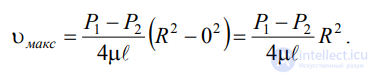
Now let us determine the fluid flow rate in laminar flow in a
circular pipe. Since the velocity distribution profile in a circular pipe
has the form of a paraboloid of revolution with the maximum velocity value at the
center of the pipe, the flow rate is numerically equal to the volume of this
paraboloid. Let us determine this volume.
The maximum velocity gives the height of the paraboloid
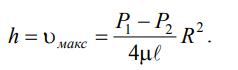
As is known from geometry, the volume of a paraboloid of height h and
base area R
2
is equal to
Velocity
profile
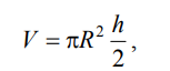
and in our case
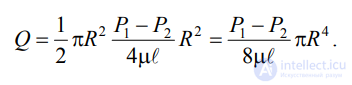 . (4.4)
If the pipe diameter d is substituted for R, formula (4.4) takes the
form
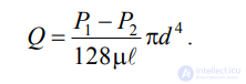 . (4.5)
The flow rate in the pipe can be expressed through the mean velocity:
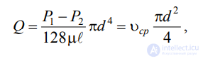
from which
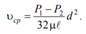 . (4.6)
To determine the head losses in laminar fluid flow in a
circular pipe, let us consider a pipe section of length , along which the flow
moves under laminar-regime conditions (Fig. 4.3). The fluid flow rate in this
pipe can be determined from formula (4.5), and the mean velocity – from
formula (4.6).
From formula (4.6), the pressure loss in the pipeline will be equal to
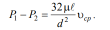 . (4.7)
If, in formula (4.6), the dynamic viscosity coefficient
is replaced by the kinematic viscosity coefficient and the density
( = ), and both sides of the equality are divided by the specific weight of the fluid = g,
we obtain:
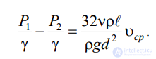
.
Since the left side of the resulting equality is equal to the head loss hloss in a
pipe of constant diameter, this equality finally takes the form:
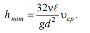 . (4.8)
The equation can be transformed into the universal Darcy–Weisbach
formula, which is finally written as:
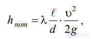 , (4.9)
where – is the coefficient of hydraulic friction, which for laminar
flow is calculated using the expression:
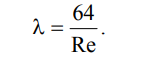 (4.10)
However, for the laminar regime, to determine the coefficient of
hydraulic friction , T.M. Bashta recommends, for Re<2300,
applying the formula
 . (4.11)
As indicated in Section 4.1, turbulent flow is characterized by
mixing of the fluid and pulsations of velocities and pressures. If
pulsations, for example, of velocity over time at a fixed point in the flow, are measured with a
sufficiently sensitive recording instrument, a
pattern similar to that shown in Fig. 4.4 is obtained. The velocity fluctuates randomly
around a certain time-averaged value, avg,
which in this case remains constant.
The character of the streamlines in the pipe at a given moment in time is
highly varied (Fig. 4.5).
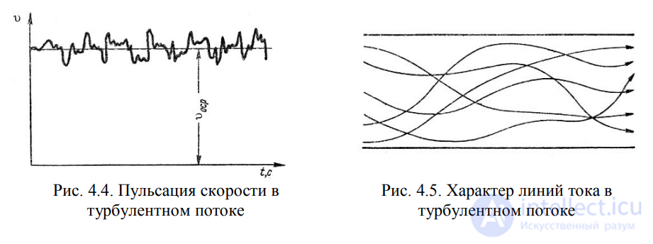
Fig. 4.4. Velocity pulsation in a turbulent flow
Fig. 4.5. Character of the streamlines in a turbulent flow
In the turbulent regime of fluid motion in pipes, the velocity
distribution profile has the form shown in Fig. 4.6. In a thin
wall layer of thickness , the fluid flows in a laminar regime, while
the remaining layers flow in a turbulent regime and are called the
turbulent core. Thus, strictly speaking, purely turbulent
motion does not exist. It is accompanied by laminar
motion at the walls, although the layer with the laminar regime is very small compared
to the turbulent core.
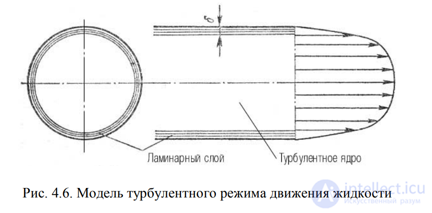
Fig. 4.6. Model of the turbulent fluid-motion regime
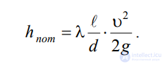
The main design formula for head losses in turbulent
fluid flow in circular pipes is the empirical formula already given
above, (4.9), known as the Darcy–Weisbach formula and
having the following form:
.
The difference lies only in the values of the coefficient of
hydraulic friction . This coefficient depends on the Reynolds number
Re and on the dimensionless geometric factor – the relative
roughness /d (or /r0, where r0 – is the pipe radius).
The first and most exhaustive work on the determination of was
carried out by I.I. Nikuradse, who, based on experimental data, plotted a
graph of lg(1000) versus lg Re for a series of values of /r0. Nikuradse's
experiments were performed on pipes with artificially imposed
roughness, obtained by gluing sand grains of a certain
size to the inner walls of the pipe. The results of these
studies are shown in Fig. 4.7, where curves of
lg (1000) versus lg Re are plotted for a series of values of /r0.
Line I corresponds to the laminar regime of fluid motion in
accordance with (4.10).
Next, three regions can be distinguished on the graph.
The first region – the region of small Re and /r0, where the coefficient does not
depend on the roughness but is determined only by the Re number (marked in
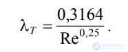
Fig. 4.7 by line II). This is the region of hydraulically smooth pipes. If the
Reynolds number lies in the range 4000 < Re < 10(d / e), the coefficient
is determined by the semi-empirical Blasius formula
 . (4.12)
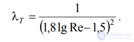
To determine there is also an empirical formula of
P.K. Konakov, which is applicable for hydraulically smooth pipes
 (4.13)
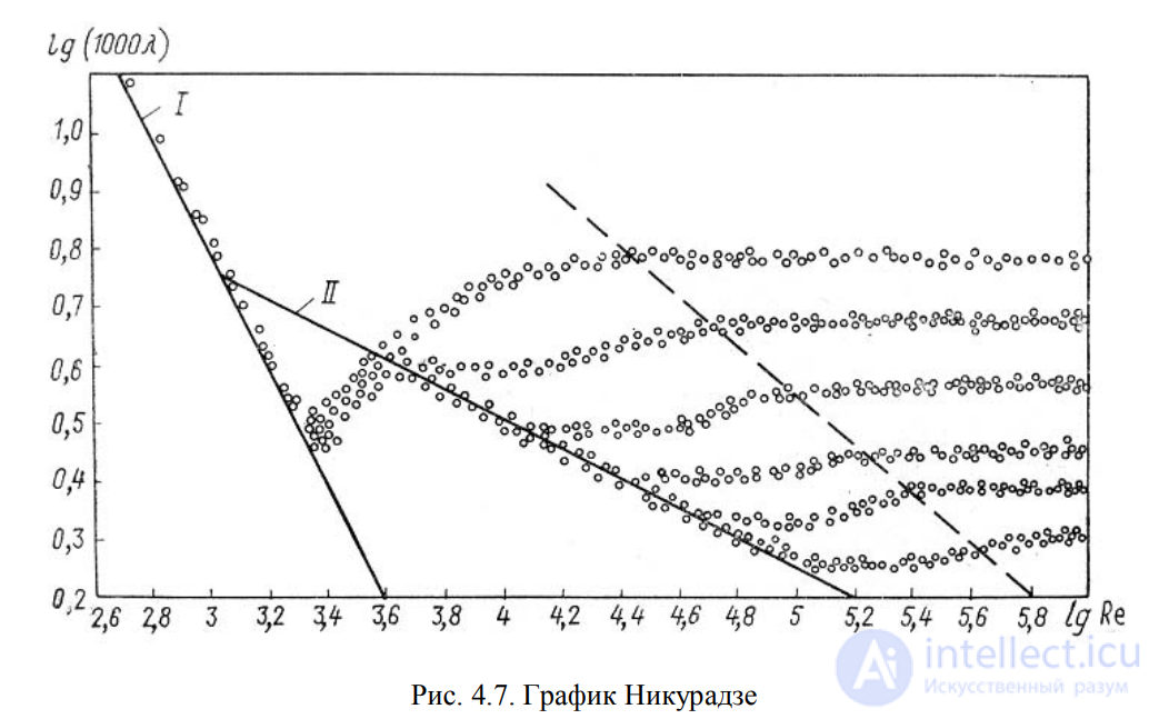
Fig. 4.7. Nikuradse diagram
In the second region, located between line II and the dashed
line on the right, the coefficient depends simultaneously on two parameters
– the Re number and the relative roughness /r0, which can be replaced
by e. To determine the coefficient in this region, the
universal formula of A.D. Altshul can be used:
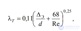 , (4.14)
where e – is the equivalent absolute roughness.
Typical values of e (in mm) for pipes made of various materials
are given below
Glass ……………………………………………………….. 0
Drawn tubing of brass, lead, copper………………….. 0…0.002
High-quality seamless steel pipes……….. 0.06…0.2
Steel pipes……………………………………………... 0.1…0.5
Asphalted cast-iron pipes……………………….. 0.1…0.2
Cast-iron pipes……………………………………………... 0.2…1.0
The third region – the region of large Re and /r0, where the coefficient does not
depend on the Re number but is determined only by the relative roughness
(the region located to the right of the dashed line). This is the region of
rough pipes, in which all lines with different roughnesses are
parallel to one another. This region is called the region of
self-similarity, or the quadratic-resistance regime, since here
the hydraulic losses are proportional to the square of the velocity.
The determination of for this region is carried out by the simplified Altshul
formula:
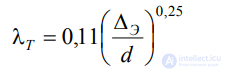 (4.15)
or by the Prandtl–Nikuradse formula:
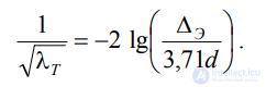 . (4.16)
Thus, the head losses, determined by the Darcy–Weisbach formula
(4.9), can be found once the coefficient of hydraulic
resistance is known, which is determined depending on the Reynolds number
Re and on the equivalent absolute roughness e. For convenience,
summary data for determining are presented in Table 4.1.
Using the formulas given in Table 4.1 to determine the
coefficient is not always convenient. To simplify calculations, one can
use the Colebrook–White nomogram (Fig. 4.8), by means of
which can be determined quite simply from the known Re and e / d.
Table 4.1
Table for determining the coefficient of hydraulic friction
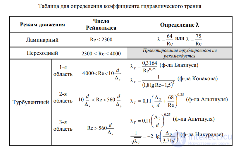
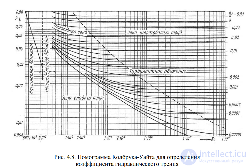
Fig. 4.8. Colebrook–White nomogram for determining
the coefficient of hydraulic friction
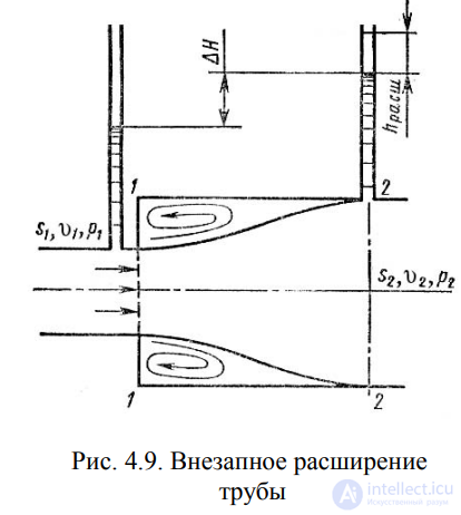
Fig. 4.9. Sudden expansion of a pipe
All hydraulic energy losses are divided into two types: friction
losses along the length of pipelines (discussed in Sections 4.3 and 4.4), and local
losses, caused by such pipeline elements in which,
due to a change in the size or configuration of the channel, there occurs
a change in flow velocity, separation of the flow from the channel walls, and the formation of
vortices.
The simplest local hydraulic resistances can be
divided into expansions, contractions, and turns of the channel, each of which
can be sudden or gradual. More complex cases of local
resistance are combinations of
the simple resistances listed above.
Let us consider the simplest local resistances under the turbulent
flow regime in a pipe.
1. Sudden expansion of the channel. The head (energy) loss at a
sudden expansion of the channel is expended on vortex formation, associated
with the separation of the flow from the walls, i.e., on sustaining the continuous rotational
motion of fluid masses with their constant renewal.
At a sudden expansion of the channel
(pipe) (Fig. 4.9), the flow separates at the corner
and expands not suddenly, as does the channel, but
gradually, with vortices forming in the annular
space between the flow and the pipe
wall, and these vortices are the
cause of the energy losses.
Let us consider two flow sections: 1-1 – in
the plane of the pipe expansion, and 2-2 – at
the point where the flow, having expanded,
has filled the entire cross-section of the wide pipe.
Since the flow expands between the sections under
consideration, its velocity
decreases while the pressure increases.
Therefore the second piezometer shows a
height H greater than the first; but
if there were no head loss at this location, the second piezometer
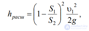
would show a height greater by an additional hexp. This height is the local head
loss due to expansion, which is determined by the formula:
 , (4.17)
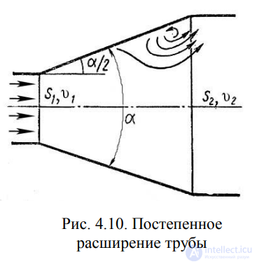
Fig. 4.10. Gradual expansion of a pipe
where S1, S2 – are the cross-sectional areas at 1-1 and 2-2.
This expression is a consequence of Borda's theorem, which states
that the head loss at a sudden expansion of the channel is equal to the velocity
head determined from the difference of the velocities
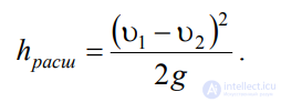 . (4.18)
The expression 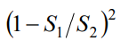 in (4.17) is denoted by the Greek letter
(zeta) and is called the loss coefficient; thus
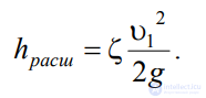 (4.19)
2. Gradual expansion of the channel. A gradually expanding
pipe is called a diffuser (Fig. 4.10). The flow velocity in a diffuser
decreases while the pressure increases, and
consequently the kinetic energy of the fluid is converted into
pressure energy. In a diffuser, just
as in a sudden expansion of the channel,
separation of the main flow from the
wall and vortex formation occur.
The intensity of these phenomena increases
with an increase in the expansion angle
of the diffuser .
In addition, the diffuser also has
ordinary friction losses, similar
to those that occur in pipes
of constant cross-section.
The total head loss in the
diffuser is considered as the sum
of two terms:
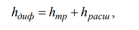 , (4.20)
where hfr and hexp are the head losses due to friction and expansion
(vortex formation), respectively.
In expression (4.20)
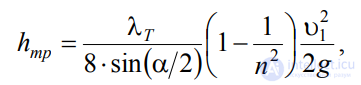 , (4.21)
where 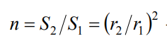 – is the degree of expansion of the diffuser.
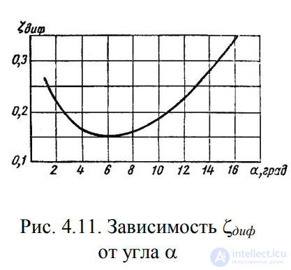
Fig. 4.11. Dependence of diff on the angle
The head loss due to expansion hexp in expression (4.20) has the same
nature as in the case of a sudden expansion of the channel
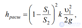 , (4.22)
where k is the softening coefficient; for = 5…20, k = sin .
Taking (4.21) and (4.22) into account, the original expression (4.20)
can be rewritten as:
 , (4.23)
from which the resistance coefficient of the diffuser can be expressed by the formula
 . (4.24)
The function 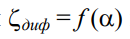 has a minimum at
a certain optimal value of the angle ,
the value of which is determined by the following
expression:
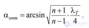 . (4.25)
Substituting into this formula
T = 0.015…0.025 and n = 2…4, we obtain
opt = 6 (Fig. 4.11).
3. Sudden contraction of the channel. In this case the head loss
is caused by friction of the flow as it enters the narrower pipe and by losses due to
vortex formation, which occur in the annular space around the
contracted part of the flow (Fig. 4.12).
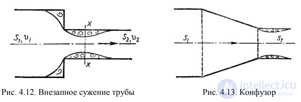
Fig. 4.12. Sudden contraction of a pipe Fig. 4.13. Confuser
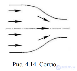
Fig. 4.14. Nozzle
The total head loss is determined by the formula;
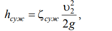 (4.26)
where the contraction resistance coefficient is determined by the
semi-empirical formula of I.E. Idelchik:
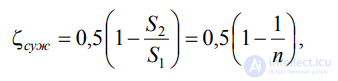 , (4.27)
in which n = S1/S2 – is the degree of contraction.
When the pipe discharges from a reservoir of large dimensions, when it can
be assumed that S2/S1 = 0, and also in the absence of rounding of the inlet corner,
the contraction resistance coefficient con = 0.5.
4. Gradual contraction of the channel. This local resistance
is a converging conical pipe, which is called a
confuser (Fig. 4.13). Fluid flow in a confuser is accompanied
by an increase in velocity and a drop in pressure. In a confuser there are only
friction losses
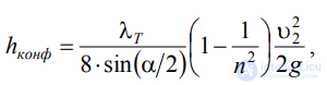 , (4.28)
where the resistance coefficient of the confuser is determined by the formula
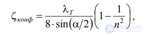 , (4.29)
in which n = S1/S2 – is the degree of contraction.
A small amount of vortex formation and separation of the
flow from the wall, with simultaneous contraction
of the flow, occurs only at the outlet from the
confuser, at the point where the conical
pipe joins the cylindrical one. By rounding the
inlet corner, the head loss at pipe entry
can be significantly reduced. A confuser with smoothly joined
cylindrical and conical parts
is called a nozzle (Fig. 4.14).
5. Sudden turn of a pipe (elbow). This type of local
resistance (Fig. 4.15) causes significant energy losses, since in
it, separation of the flow and vortex formation occur, and the losses are
greater the larger the angle . The head loss is calculated by the formula
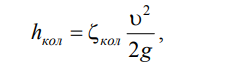 , (4.30)
where elbow – is the resistance coefficient of a round-section elbow,
which is determined from a graph as a function of the elbow angle
(Fig. 4.16).
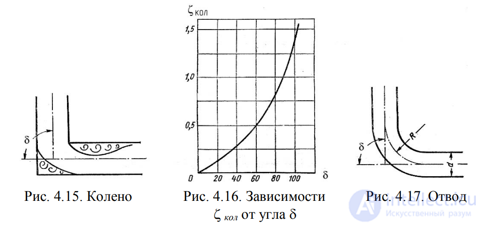
Fig. 4.15. Elbow Fig. 4.16. Dependence of elbow on the angle Fig. 4.17. Bend
6. Gradual turn of a pipe (rounded elbow or bend).
The smoothness of the turn significantly reduces the intensity of
vortex formation, and consequently the resistance of the bend compared
to the elbow. This reduction is greater the larger the relative
radius of curvature of the bend R / d (Fig. 4.17). The resistance coefficient of the
bend, bend, depends on the ratio R / d, the angle , and also on the shape of the cross
section of the pipe.
For bends of circular cross-section with an angle = 90 and R / d ≥ 1, in
turbulent flow, the empirical formula can be used:
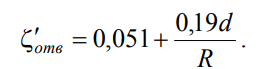 . (4.31)
For angles < 70, the resistance coefficient is
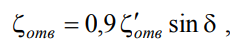 , (4.32)
and for > 100
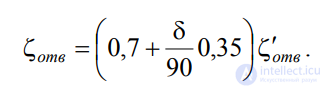 . (4.33)
The head loss in the elbow is determined as
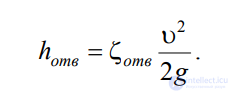 . (4.34)
Everything stated above relates to turbulent fluid
motion. In laminar motion, local resistances play a
minor role in determining the overall resistance of the pipeline. In addition,
the resistance law for the laminar regime is more
complex and has been studied to a lesser extent.

Comments