
Lecture
Hydrodynamics – a branch of hydraulics that studies the laws
of fluid motion and its interaction with stationary and moving
surfaces.
If the individual particles of an absolutely rigid body are rigidly connected
to one another, then in a moving fluid medium such connections are absent.
The motion of a fluid consists of an extremely complex displacement
of individual molecules.
The cross-sectional area (m2
) is the area of the cross section
of the flow, perpendicular to the direction of flow. For example, the cross
section of a pipe is a circle (Fig. 3.1, b); the cross section of a valve is a ring with
a variable inner diameter (Fig. 3.1, b).
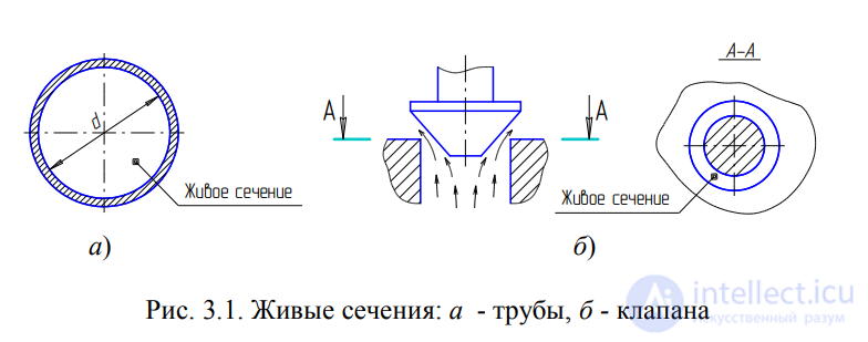
Fig. 3.1. Cross sections: a – pipe, b – valve
The wetted perimeter («chi») is the part of the perimeter of the cross section
bounded by solid walls (Fig. 3.2, shown by the thickened line).
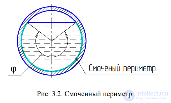
Fig. 3.2. Wetted perimeter
For a circular pipe
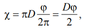 if the angle is in radians,
or
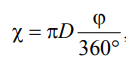 , if the angle is in degrees.
Flow rate Q – the volume of fluid V flowing per unit
time t through the cross section .
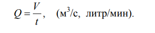 . (3.1)
Mean flow velocity – the velocity of fluid motion,
determined as the ratio of the fluid flow rate Q to the cross-sectional
area
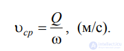 . (3.2)
Since the velocity of motion of different fluid particles
differs from one another, the velocity of motion is therefore averaged. In a
circular pipe, for example, the velocity at the pipe axis is maximum, whereas at
the pipe walls it is equal to zero.
The hydraulic radius of the flow R – the ratio of the cross-sectional area to the
wetted perimeter
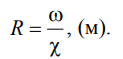 , (m). (3.3)
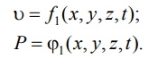
Fluid flow can be steady or
unsteady. Steady motion is the
motion of a fluid in which, at a given point of the channel, the pressure and
velocity do not change with time
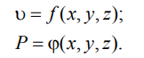
Motion in which the velocity and pressure change not only
with spatial coordinates but also with time is called
unsteady, or non-stationary
A streamline (used for unsteady motion) is a
curve at every point of which the velocity vector at a given instant of time
is directed tangentially.
A stream tube – a tubular surface formed by streamlines with an
infinitesimally small cross section. The part of the flow enclosed
inside the stream tube is called an elementary filament.
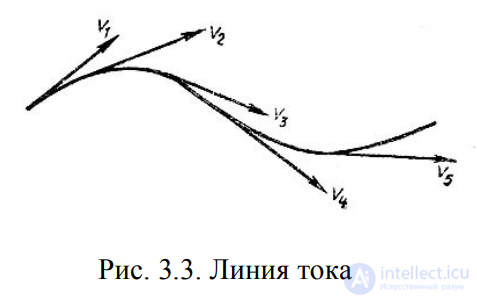
Fig. 3.3. Streamline
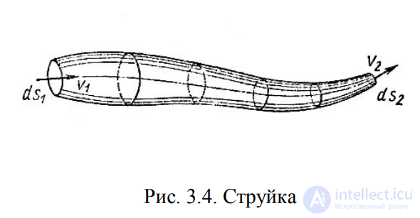
Fig. 3.4. Filament
Fluid flow can be pressurized or free-surface (gravity) flow. Pressurized
flow is observed in closed channels without a free surface.
Pressurized flow is observed in pipelines with elevated
(or reduced) pressure. Free-surface flow – flow with a free
surface, which is observed in open channels (rivers, open
canals, flumes, etc.). This course will consider only
pressurized flow.
From the law of conservation of matter and constancy of flow rate, the
continuity equation for flows is derived. Consider a pipe with a variable
cross section (Fig. 3.5). The flow rate of fluid through the pipe at any of its
cross sections is constant, i.e., Q1 Q2 = const, from which
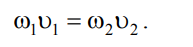
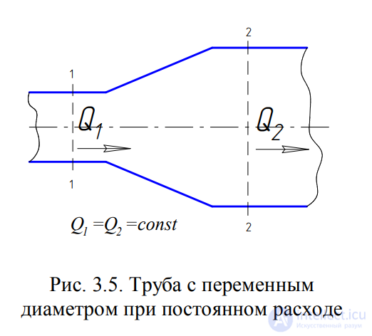
Fig. 3.5. Pipe with variable diameter at constant flow rate
.
Thus, if the flow in the
pipe is continuous and
unbroken, the continuity
equation takes the form:
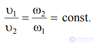 (3.4)
(3.4)
Daniel Bernoulli's equation, obtained in 1738, is a
fundamental equation of hydrodynamics. It provides a relationship between
pressure P, mean velocity , and piezometric height z at
various cross sections of the flow and expresses the law of conservation of energy
of a moving fluid. This equation is used to solve a large
range of problems.
Consider a pipeline of variable diameter, positioned in
space at an angle (Fig. 3.6).
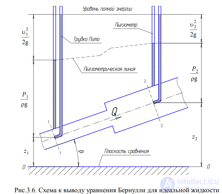
Fig. 3.6. Diagram for the derivation of Bernoulli's equation for an ideal fluid
Let us arbitrarily choose two cross sections along the pipeline segment under consideration:
section 1-1 and section 2-2. Fluid moves up the pipeline from the first
section to the second, with flow rate equal to Q.
To measure the pressure of the fluid, piezometers are used –
thin-walled glass tubes in which the fluid rises to a
height

. A piezometer is installed at each section, in which
the fluid level rises to different heights.
In addition to the piezometers, a tube is installed at each section, 1-1 and 2-2,
with its bent end directed against the flow of the fluid, which
is called a Pitot tube. The fluid in the Pitot tubes also rises to
different levels, if measured from the piezometric line.
The piezometric line can be constructed as follows.
If several such piezometers are placed between section 1-1 and 2-2
and a curve is drawn through the fluid level readings in them, we
obtain a broken line (Fig. 3.6).
However, the height of the levels in the Pitot tubes relative to an arbitrary
horizontal line 0-0, called the datum plane, will be
the same.
If a line is drawn through the fluid level readings in the Pitot tubes,
it will be horizontal and will reflect the level of the total
energy of the pipeline.
For two arbitrary sections 1-1 and 2-2 of a flow of an ideal
fluid, Bernoulli's equation has the following form:
 (3.5)
(3.5)
Since sections 1-1 and 2-2 are taken arbitrarily, the equation
obtained (3.5) can be rewritten differently:
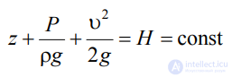 (3.6)
(3.6)
and read as follows: the sum of the three terms of Bernoulli's equation for any
cross section of a flow of an ideal fluid is a constant value.
From an energy standpoint, each term of the equation represents
a certain type of energy:
z1 and z2 – specific energies of position, characterizing
the potential energy at sections 1-1 and 2-2;
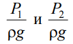 - specific pressure energies, characterizing the
potential energy of pressure at the same sections;
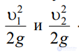
- specific kinetic energies at the same sections.
Consequently, according to Bernoulli's equation, the total specific
energy of an ideal fluid at any cross section is constant.
Bernoulli's equation can also be interpreted purely geometrically.
The fact is that each term of the equation has a linear dimension.
Looking at Fig. 3.6, one can notice that z1 and z2 are the geometric heights
of sections 1-1 and 2-2 above the datum plane;
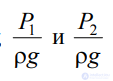
- the piezometric
heights;
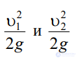
- the velocity heads at the indicated sections.
In this case, Bernoulli's equation can be read as follows: the sum of the
geometric, piezometric, and velocity heads for an ideal
fluid is a constant value.
Bernoulli's equation for the flow of a real fluid differs somewhat
from equation (3.5).
The fact is that when a real viscous fluid moves, friction
forces arise, to overcome which the fluid expends energy. As a
result, the total specific energy of the fluid at section 1-1 will be greater than
the total specific energy at section 2-2 by the amount of energy lost
(Fig. 3.7).
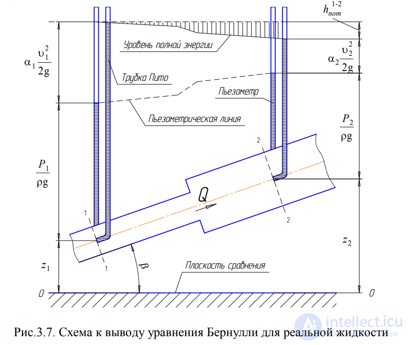
Fig. 3.7. Diagram for the derivation of Bernoulli's equation for a real fluid
The lost energy, or head loss, is denoted 12 hloss and also has a linear dimension.
Bernoulli's equation for a real fluid takes the form:
 (3.7)
(3.7)
From Fig. 3.7 it can be seen that as the fluid moves from section 1-1 to
section 2-2, the lost head continuously increases (the lost
head is shown by vertical hatching). Thus, the level of the
initial energy possessed by the fluid at the first section, at
the second section, will be composed of four components:
geometric height, piezometric height, velocity head, and
lost head between sections 1-1 and 2-2.
In addition, two more coefficients, 1 and 2, appear in the equation,
which are called Coriolis coefficients and depend on the
flow regime ( = 2 for laminar flow, = 1 – for
turbulent flow1
).
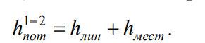
The lost head 12
hloss consists of linear losses,
caused by friction between the layers of fluid, and losses caused by
local resistances2
(changes in flow configuration)
loss linear local
.
Bernoulli's equation is used to solve most problems
in practical hydraulics. To do this, two sections are chosen along the length of the
flow, such that for one of them the quantities
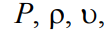 are known, while for the other section one or more quantities are to be determined.
When there are two unknowns for the second section, the equation of
constancy of fluid flow rate is used 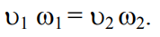
To measure the velocity at points in a flow, a Pitot tube
(Fig. 3.8), which operates on the principle of Bernoulli's equation, is widely used;
its bent end is directed against the flow. Suppose it is required to
measure the fluid velocity at some point in the flow. By placing the end of the
tube at the indicated point and writing Bernoulli's equation for section I-I and
the section passing at the level of the fluid in the Pitot tube, we obtain

1 Flow regimes are discussed in Lecture No. 4
2 Local resistances of pipelines are discussed in Lecture No. 4
where H – the column of fluid in the Pitot tube.
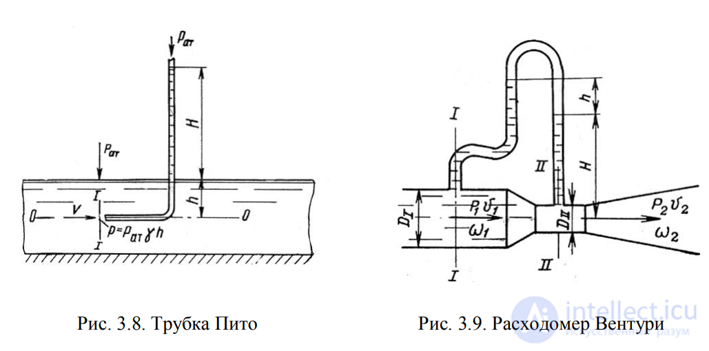
Fig. 3.8. Pitot tube Fig. 3.9. Venturi flow meter
To measure the fluid flow rate in pipelines, a
Venturi flow meter is often used, whose operation is likewise based on the principle of
Bernoulli's equation. The Venturi flow meter consists of two conical
sections with a cylindrical insert between them (Fig. 3.9). If
piezometers are placed at sections I-I and II-II, the difference in levels in them will
depend on the flow rate of the fluid flowing through the pipe.
Neglecting head losses and taking z1 = z2, we write Bernoulli's
equation for sections I-I and II-II:
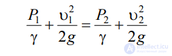
or
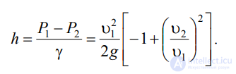
Using the continuity equation
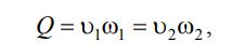
,
we substitute into the resulting expression:
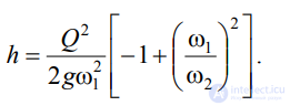
Solving for Q, we obtain
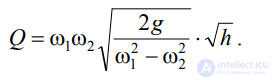
.
The expression preceding h is a constant
quantity, called the Venturi meter constant.
From the equation obtained, it can be seen that h depends on the flow rate Q. This
relationship is often plotted as a calibration curve of h versus Q, which has
a parabolic character.

Comments