
Lecture
From history. Many decompositions of a special kind are widely known. The relevance of such methods is confirmed, for example, by the history of the famous strong Berge conjecture (1962), which held for 40 years and was proved in 2002 on the basis of decomposition methods.
A decomposition of a graph is a covering of it by parts satisfying certain special conditions. The conditions may be completely different and are determined by the problems the decomposition is aimed at solving.
A distinction is made between the classical decomposition of graphs and the algebraic decomposition of graphs.
Let us consider the algebraic decomposition of graphs. The algebraic nature of the new decomposition theory consists in the fact that the set of graphs is turned into an algebraic system with a semigroup of operators acting on it. Multiplication in the semigroup is category-theoretic: operators are multiplied as morphisms. The operators are, roughly speaking, the graphs themselves. In general algebra this is an old, tried-and-true idea, but in graph theory it is a new phenomenon. The result of these constructions is a decomposition of an arbitrary graph into parts, «similar» to the canonical factorization of a natural number, which is why the new decomposition is called canonical.
In graph theory, a branch decomposition of an undirected graph G — is a hierarchical clustering of the edges of the graph G, represented by an unrooted binary tree T with the edges of G as its leaves. Removing any edge from T divides the edges of the graph G into two subgraphs, and the width of the decomposition is taken to be the maximum number of shared vertices in any subgraph obtained in this way. The branchwidth of a graph G — is the minimum width of any branch decomposition of the graph G.
Branchwidth is closely related to treewidth — for all graphs they are within a constant factor of each other, and both quantities can be characterized by forbidden minors. As with treewidth, many optimization problems on graphs can be solved efficiently on graphs of small branchwidth. However, unlike treewidth, the branchwidth of a planar graph can be computed exactly in polynomial time. Branch decomposition and branchwidth can be generalized from graphs to matroids.
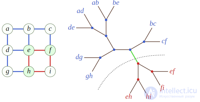
Branch decomposition of a grid. An e-separation is shown. The separation, the decomposition, and the graph itself have width three.
A path (route, Eng. path) in a graph is a sequence of the form  — the length (Eng. length) of the path.
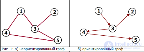
A path in a graph is a finite sequence of vertices in which every two consecutive vertices are connected by an edge. A path may be directed or undirected depending on the graph. In fig. 1.a, a path is, for example, the sequence [(1), (4), (5)]; in fig. 1.b, [(1), (3), (4), (5)].
The length of a path — the number of edges included in the sequence that defines this path.
A closed path (Eng. closed walk) in a directed graph is a path in which v0=vk
A closed path in an undirected graph is a path in which 
A cycle (Eng. integral cycle) — is an equivalence class of closed paths under an equivalence relation such that two paths are equivalent if
 — are two sequences of edges in a closed path.
A simple (vertex-simple) path (Eng. simple path) — a path in which each of the vertices of the graph occurs at most once.
An edge-simple path — a path in which each of the edges of the graph occurs at most once.
A path for which no edges of the graph connect two vertices of the path is called an induced path.
A simple chain containing all vertices of the graph without repetition is known as a Hamiltonian path.
A simple cycle containing all vertices of the graph without repetition is known as a Hamiltonian cycle.
A cycle obtained by adding an edge of the graph to a spanning tree of the original graph is known as a fundamental cycle.
Two paths are vertex-independent if they have no internal vertices in common. Similarly, two paths are edge-independent if they have no internal edges in common.
The length of a path — is the number of edges used in the path, where repeatedly used edges are counted the corresponding number of times. The length may be zero if the path consists of a single vertex.
A weighted graph associates with each edge a certain value (the edge weight). The weight of a path in a weighted graph is the sum of the weights of the edges of the path. Sometimes instead of the word weight the words cost or length are used.
The shortest path problem — the problem of finding the shortest path (chain) between two points (vertices) in a graph, in which the sum of the weights of the edges making up the path is minimized.
The shortest path problem is one of the most important classical problems of graph theory. Today many algorithms are known for solving it[⇨].
This problem also has other names: the minimum path problem or, in an outdated form, the stagecoach problem.
The significance of this problem is determined by its various practical applications[⇨]. For example, GPS navigators perform a search for the shortest path between two intersections. The intersections serve as vertices, and the roads are the edges that lie between them. If the sum of the lengths of the roads between the intersections is minimal, then the path found is the shortest.
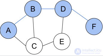
The shortest path (A, B, D, F) between vertices A and F in an undirected unweighted graph.
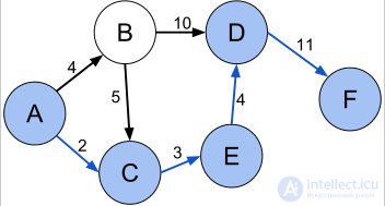
The shortest path (A, C, E, D, F) between vertices A and F in a weighted directed graph.
General theory:
We have a graph G=(V,E), where the connection between vertices v and w is as follows: a(v,w)  E. If there is no connection between the vertices, then a(v,w)=
 .
.
If the last vertex wo, w1, …, wn defines a path in the graph, then its length equals the total weight of the included vertices:
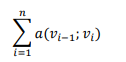
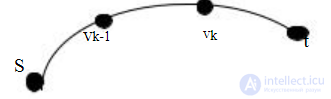
Our task – finding the shortest path between vertices S, t. M(S,t) – the distance between S and t. The path from S to t that has the minimum length – is the shortest path between vertices S and t. d(S,t)=d(S,vk) + a(vk,t)
d(S,vk)=d(S,vk-1)+a(vk-1,vk)
Finding the shortest path in an acyclic graph:
An acyclic digraph (Acyclic graph, DAG) — a digraph containing no contours but possibly having cycles (see cycle in a digraph). In English-language literature it appears as the abbreviation DAG from Directed Acyclic Graph.
Hence another name — Acyclic graph, DAG.
example of an acyclic graph
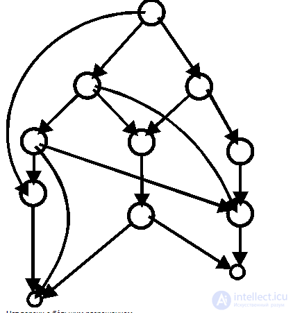
Finding the shortest path in an acyclic graph has 2 parts. The first is renaming the vertices of the graph so that the first vertex has no incoming vertices. The second part is the search for the shortest paths itself.
To begin, let us specify an arbitrary acyclic graph with arbitrary numbering and weights.
And let us write it in the form of an adjacency matrix, where edges that do not enter other edges will be marked with the maximally large number 32767.
To renumber the graph so that vertex No. 1 has only outgoing edges, we use the Topolsoft algorithm.
Topolsoft algorithm (G,N)
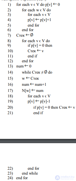
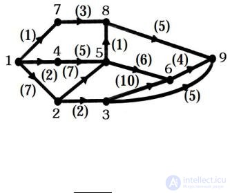
After which we obtain the following numbering of the graph.
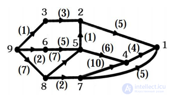
Algorithm for finding the shortest paths.
After that, one can find the shortest distances from vertex No. 1 to each of the vertices using the DSP algorithm.
DSP algorithm (G, N, d)
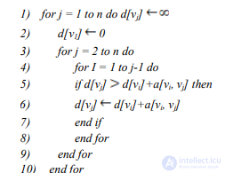
After that we output the result to the screen. In this case we compute the computational complexity as follows:
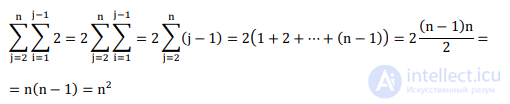
And it will be: O(n2)
The decomposition problem is formulated as follows: a graph is given for which it is necessary to determine whether it is the product of two graphs. In the case of a positive answer, one must find the factor graphs.
Semantics of the problem. A system functioning over time is described. It is necessary to determine whether it can be represented as a system of two independent blocks, as described above. In this case the system can be described much more simply. Thus, if the system has 100 states, then with a positive solution it will be described as two blocks, each of which has only ten states.
It was shown earlier that if a graph is representable as a product, then its matrix will have the form of a proper block matrix.
Let us once again consider the example given in the previous section in table 3.10.
Suppose that in the system the states are numbered as follows:
1=(1aa), 2=(1bb), 3=(3bb), 4=(2bb), 5=(3aa), 6=(2aa), that is, we swap the 3rd
and 6th vertices. Then the table takes the form. We obtain table 3.11.
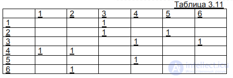
This table will no longer be a proper block matrix, although it describes a graph that coincides with the original one up to the names of the vertices.
This means that if the matrix of a graph is not a proper block matrix but can be obtained from one by renaming vertices, then such a graph will represent a product of graphs.
There is one more simple criterion that a graph is not a product. If Q=<C,T>, G=<A,R>, H=<B,S>, and Q=GxH, then the condition holds:
|C|=|A|×|B|. Hence, if the number of vertices n of a graph is a prime number, then it cannot be represented as a product of graphs.
If n is not prime and can be expressed as n=kr , where k and r are greater than 1, then one can pose the problem of checking this graph for the possibility of representing it as a product. If a graph contains n vertices, then to check it one must in the general case perform n! renamings. Already for n=6 this number will be 720, and for n=8 already more than 40000. Therefore there arises the need to reduce the volume of computations.
The possibility of reduction is based on the following statement. If a graph is represented as a proper block matrix, then upon renaming vertices associated with renaming vertices in one factor graph, the matrix will remain a proper block matrix. Likewise, if the matrix is not a proper block matrix, then a permutation of names associated with a change of names in one factor graph will not make it proper. This means that if n=k×r, then the necessary enumeration of variants can be reduced by a factor of k!×r!. For example, the enumeration for n=6 is reduced to 60 (6=2×3, a reduction by a factor of 2!×3!=12).
Decomposition algorithm
Let us once again consider the product operation. If vertex a in the first factor graph has in-degree Da, and vertex b in the second graph has in-degree Db, then in the resulting graph the vertex (a,b) will have in-degree (DaDb). The same can be said about the out-degree of the resulting graph.
The algorithm is based on the fact that for each i-th vertex of the graph all possible factorizations of its in-degrees si=ri×ti are determined, i.e. it is assumed that if the problem is solvable and this vertex is matched with a pair (x,y), then these vertices have in-degrees ri and ti respectively. The same applies to the out-degree of vertex i: ti=pi×qi.
Let us carry out the factorizations for all degrees of the vertices. Let us construct two partitions of the vertices: a partition into k classes of l elements p=(p1,p2,…,pk) and a partition into l classes of k elements r=(r1, r2, …, rl), n=k×l, so that the product of these partitions is the partition into singleton sets.
Vertices a and b fall into one class p if for them in the factorization raa=rbb and paa=pbb.
Vertices a and b fall into one class r if in the factorizations taa=tb and qa=qb.
If such partitions can be constructed, then it is matched with a permutation of elements according to the following rule. Let us fix the order of the blocks in the partitions p and r. Let us match this order with a permutation: first the priority is determined by the partition p, then within these blocks by the partition r.
Let us consider the method by example. Let the graph be described by the matrix of table 3.12; the factorizations of s and t are given in this table. A degree value equal to 0 is represented by the product of 0 and an arbitrary number denoted as x. The first task is the task of selecting, among the factorizations, those that will lead to partitions of the vertices by out-degree and in-degree.
When selecting factorizations we will take the following into account.
For vertex 4 we choose the partition 2×2, since a partner for a vertex with factor 4 cannot be found. In the factorization p, vertices 4 and 5 must be in different blocks, since both of their components by s are different. The same holds with respect to t for vertices 3 and 4. Hence, 3 and 5 will be in one block. Vertices 3 and 6 must be in one block by t and in different blocks by s, 1 and 5 – in different blocks by t, so that by the first component they can be combined in the factorization r. The partitions are set in italics. As a result we obtain the factorization p={{1,4,6}, {2,3,5}}.
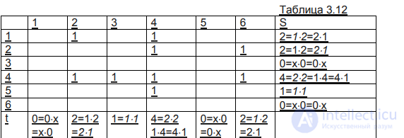
After this we uniquely obtain r={{1,5},{3,6},{2,4}}.
Let us fix the order in these partitions. We thereby assume that if a solution exists, then the graph can be represented as a product of two graphs, one of which contains 2 vertices (let, for example, vertices a and b), and the second contains three vertices (let, for example, 1, 2 and 3). Then the vertices of the first block of the partition p are matched with the elements of the Cartesian product with vertex a as the first summand, and for the vertices of the second block the first summand will be b.
Similarly, in the corresponding Cartesian product, the second factor for the vertices of the first block of the partition r will be vertex 1, for the second block – vertex 2, and for the third block – vertex 3. Let us form for the partitions p and r the ordering <1,4,6,5,2,3>, which «spoiled» the matrix; we correct it using the inverse ordering
1 2 3 4 5 6
1 5 6 2 4 3.
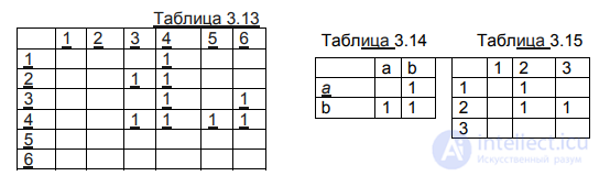
Let us apply this permutation to the matrix; we obtain table 3.13. As can be seen from the table, it is a proper block matrix, which leads to the solution: the graph is representable as a product of two graphs, whose adjacency matrices are easily obtained from table 3.13. The matrices of the factor graphs are presented in tables 3.14 and 3.15.
Example of assignments
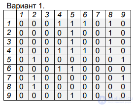
For a given graph, determine whether it is decomposable into a product of two graphs. If it is decomposable, then find the factor graphs.
Distinctive features of the graphs arising in modern applications are their large dimensionality and sparsity. Speeding up the operation of any of the known algorithms for solving optimization problems on graphs can be achieved through preprocessing of the original graph. The preprocessing technology is implemented, as a rule, in the form of a two-phase procedure. In the first phase the graph is preprocessed by reducing or decomposing it. The choice of the type of preprocessing is determined by the features of the problem being solved and the structure of the graph. In the second phase, a known algorithm for solving the problem is usually applied to the transformed graph and a solution for the original graph is formed. It is required that the preprocessing substantially reduce the dimensionality of the problem, ensure the correctness of forming the solution of the problem based on one or several solutions obtained for the transformed graph, and that the computational complexity of the preprocessing not exceed the complexity of solving the problem under consideration on the original graph.
The implementation of the decomposition approach, that is, the process of extracting parts of the original graph, largely depends on the structural features of this graph, including the constraints on the parameters characterizing its sparsity. One of the sparsity parameters of a graph is a constraint on its treewidth [1, 2]. For graphs with bounded treewidth, a decomposition of the graph by clique minimal separators is used. The idea of such a decomposition was proposed by R. Tarjan as a means of implementing the «divide and conquer» principle for solving NP-hard problems on graphs based on the adjacency relations of the graph's vertices. The parts of the graph obtained as a result of the decomposition were called atoms. Tarjan established that the decomposition of a graph into atoms does not destroy the cliques of this graph, does not generate new cliques, and in this sense preserves its structure.
In this work, algorithms and programs are proposed that practically implement Tarjan's idea. The application of this approach to the NP-hard clique problem is demonstrated.
Basic concepts and notation
Let us introduce the basic concepts and notation from graph theory necessary for presenting the results of the work. We use the terminology and notation adopted in the work.
Let G = (V, E) be an undirected finite graph with a set of vertices V and a set of edges E. Vertices v1 and v2 of the graph G are considered adjacent if {v1, v2} Î E, and non-adjacent otherwise. An edge e is incident to vertex v1 if e = {v1, v2} Î E, and not incident otherwise. If e = {v1, v2} Î E, then vertices v1 and v2 are called the endpoints of edge e. In this case it is also said that edge e connects vertices v1 and v2. Two edges are considered multiple if their endpoints coincide. An edge connecting a vertex to
itself is called a loop. A simple graph – an undirected finite graph G = (V, E) without loops
and multiple edges. Everywhere below only simple graphs will be considered, for which ½V½ ³ 2 and ½E½ ³ 1.
The set of all vertices of the graph G adjacent to some vertex v Î V forms in G the neighborhood (or open neighborhood) of vertex v, which is denoted by N(v). The closed neighborhood of vertex v is denoted N[v] and is defined by the equality: N[v] = N(v) È {v}. The number deg v = | N(v) | is called the degree of vertex v.
A graph G¢ = (V¢, E¢) is called a subgraph of the graph G = (V, E) provided that V¢ Í V, E¢ Í E. A subgraph G¢ = (V¢, E¢) is spanning when V¢ = V. If the set of vertices of the subgraph G¢ is V¢, and the set of its edges coincides with the set of all edges of the graph G both endpoints of which belong to V¢, then G¢ is called the subgraph induced by the set V¢ Í V, and is denoted G(V¢). Every maximal connected subgraph of the graph G, with respect to inclusion, forms its connected component. The set of vertices of some component of the graph G is called a connectivity region of this graph.
A set of vertices V¢ is called a clique of the graph G if in the graph G(V¢) every two vertices are adjacent, and a maximal clique if it is not contained in a clique with a larger number of vertices. The size of the largest (by number of vertices) clique of the graph G is denoted j(G) and is called the density of the graph G. A graph G = (V, E) that is a clique is called a complete graph and is denoted by Kn, where n = ½V½. For it j(Kn) = ½V½, and in the general case for G = (V, E) always 1 £ j(G) £ ½V½.
It is said that a set of vertices S Ì V separates non-adjacent vertices u and v of the graph G = (V, E) if
in the graph G - S = G(V \ S) the vertices u and v belong to different connected components. The set S is then called a (u, v)-separator and a minimal (u, v)-separator if S is a (u, v)-separator and it has no proper subset that is a (u, v)-separator. A separator S is considered minimal if in the graph G there exists a pair of vertices u and v such that S is a minimal (u, v)-separator. The smallest by cardinality separator of the graph G is the smallest separator. A single-vertex separator is called an articulation point of the graph. A clique minimal separator – is a minimal separator that is a clique.
A graph G is called chordal if none of its induced subgraphs is a simple cycle of length l ³ 4. Any graph can be turned into a chordal one by adding to it some set of edges. A triangulation of the graph G = (V, E) is a chordal graph H = (V, E¢), E Í E¢, which contains G as a spanning subgraph. A triangulation H is a minimal triangulation of the graph G if for G there exists no other triangulation that is a proper subgraph of the graph H. The smallest triangulation is considered to be the one with the smallest number of edges.
Treewidth – a numerical parameter characterizing the measure of tree-likeness of a graph, that is, its closeness to a tree. Treewidth is computed through a decomposition tree. By a decomposition tree of the graph G = (V, E) is meant a pair (V, T) specifying a certain partition of the vertices and edges of the graph G, where V = {Vi : i Î I} – is a family of nonempty subsets of the set V, called «bags», T = (I, W) – is a tree whose nodes are matched with these «bags». This partition satisfies the following properties [1, 2]:
The width of the decomposition tree (M, T) – is the largest capacity of its «bag», decreased by one: max{|Xi | − 1 : i Î I}. The treewidth of the graph G is defined as the smallest width of all admissible decomposition trees of it and is denoted tw(G).
Characterization of sparse and chordal graphs
Several formal definitions of a sparse graph are known. A connected graph G = (V, E), n = |V | ³ 2, |E | ³ 1, is called (edge-)sparse if the number of its edges satisfies the condition
|E| £ anb, (1)
where a > 0, 1 £ b < 2 are positive real constants. It is considered that the smaller the value of b, the more sparse the graph G is. For comparison: in every tree the number of edges equals n – 1, that is, b = 1, which corresponds to the lower bound of the value of b, and for any complete n-vertex graph always |E| = n(n – 1) /2, that is, b = 2, which corresponds to the upper bound of the value of b.
There is another definition of a sparse graph G, which is expressed through the treewidth tw(G) of this graph. For tw(G) the bounds hold: 1 £ tw(G) £ n – 1. Thus, every n-vertex tree (n ³ 2) has unit treewidth, which corresponds to the lower bound for tw(G), and a complete
n-vertex graph is characterized by treewidth equal to n – 1, which corresponds to the upper bound for tw(G). Let k be some given positive integer constant. If tw(G) £ k, then it is said that the graph G = (V, E) has bounded (by the value k) treewidth. It is considered that the smaller the value of k, the more sparse the graph G is. It is known, if tw(G) £ k, then for the number of edges of the graph G = (V, E) the inequality holds
|E| £ kn – k(k + 1) /2. (2)
For k = 1 and k = n – 1 relation (2) leads to inequalities (1), corresponding to trees and complete graphs. Consequently, the constraint tw(G) £ k does not contradict (1) and defines a natural measure of sparsity of the graph G. Considering that always j(G) – 1 £ tw(G), one can say that the value tw(G) bounds not only the number of edges of the graph but also the sizes of its cliques. In what follows the sparsity of the graph G is understood in the sense of the constraint tw(G) £ k.
The process of decomposing a graph into atoms is based on the properties of chordal graphs. Let us formulate the most important of them in the form of lemmas 1–4.
Lemma 1. A graph G = (V, E) is chordal if and only if any of its minimal separators forms a clique in G.
Lemma 2. A connected graph G = (V, E) is chordal if and only if for it there exists a clique tree, defined as follows: the set of nodes of the tree is the set {Ci : i Î J} of all maximal cliques of the graph G; two nodes Ci, Cj are connected by an edge if the corresponding cliques of the graph G have a nonempty intersection, that is, Ci Ç Cj ¹ Æ; for any vertex v Î V of the graph G the set of maximal cliques containing this vertex induces a connected subgraph that is a subtree of the clique tree.
Since every connected chordal graph G = (V, E) has no more than n - 1 maximal cliques, then, according to lemma 2, its clique tree contains no more than n - 1 nodes, where n = |V |.
Lemma 3. A connected chordal graph G = (V, E) may have several different clique trees, but each of them – is a maximum-weight spanning tree of the intersection graph of all maximal cliques of the original graph, where the weight of an edge is the number of vertices forming the intersection of the appropriate maximal cliques of the graph G.
Lemma 4. Let T – be some clique tree of a connected chordal graph G. For an arbitrary edge of the clique tree T connecting nodes Ci and Cj, the intersection Ci Ç Cj forms a minimal separator of the graph G. The converse statement is also true: if S – is a minimal separator of the graph G, then in T there will always be found an edge connecting nodes Ci and Cj such that Ci Ç Cj = S.
According to lemmas 2 and 4, in a chordal graph G = (V, E) there are no more than n - 2 minimal separators. By lemma 1 all these separators are clique separators.
Formulation of the problem of decomposing a graph into atoms
The problem of decomposing a graph into atoms (Decomposition of Graph into Atoms Problem, DGAP) can be formulated as follows:
Decomposition of Graph into Atoms Problem.
Given: a connected graph G = (V, E), for which ½V½ ³ 2, ½E½ ³ 1, tw(G) ≤ k, that is, the treewidth is bounded by some small-valued constant k > 0, as well as the set of all clique minimal separators D(G) of this graph.
Required: to find for G a set of atoms W(G) = {G1, G2, ..., Gp}, where each atom Gi, i = 1, …, p, is defined as a maximal connected subgraph of the graph G having no clique minimal separators of the graph G.
The set W(G) is customarily called the atomic representation (or decomposition into atoms) of the graph G.
It has been proved [3, 5] that the DGAP problem is polynomially solvable and has a unique solution. The latter means that the set of atoms W(G) is unique for G if the decomposition is carried out on the basis of D(G) - the set of all clique minimal separators of the graph G. If D(G) contains minimal separators that are not cliques in G, then W(G) may depend both on the composition of D(G) and on the order of examining the separators in the process of decomposition. It should be noted that the number of minimal separators of a graph is, as a rule, greater than the number of its clique minimal separators, and equality holds only for chordal graphs. In the general case a graph G = (V, E) may have an exponential number of minimal separators relative to n = |V|, whereas in a chordal graph there are always no more than n - 2 of them. Note that clique minimal separators may intersect as sets of vertices. Nesting of clique minimal separators one within another is possible, since each of them may be minimal relative to different pairs of vertices of the graph. It is noteworthy that not every graph possesses separators, including clique minimal separators: for example, there are no separators in a complete graph.
It should be noted that the atomic representation W(G) of the graph G = (V, E) is a generalization of its decomposition into blocks: when the set of clique minimal separators D(G) consists only of the articulation points of the graph G, then each atom of W(G) represents a block of this graph. Recall that a block of a graph – is a maximal, with respect to inclusion, connected subgraph of the graph G having no articulation points.
Methods for computing clique minimal separators
To determine the unique set of atoms W(G) of a given graph G = (V, E), one must first find the set D(G) of all clique minimal separators of the graph G. Such a set of separators is easily computed for a chordal graph using lemmas 1–4. However, in the general case there are two ways of finding D(G):
– find all minimal separators, and then single out among them those that form cliques in G;
– extract the clique minimal separators from a minimal triangulation H of the graph G.
Let us first consider the first method. It is known that a set S Í V is a minimal separator of the graph G = (V, E) if and only if there exist two different connectivity regions D1 and D2 of the graph G - S such that
N (D1) = N (D2) = S, (3)
N (Di) = (È v Î Di N (v)) \ Di, i = 1, 2.
Recall that the graph G - S is obtained from G by removing all vertices from S Í V. The necessary and sufficient condition (3) makes it possible to find in the graph G all minimal separators through close separators. A minimal (u, v)-separator S for which S Í N(v) is called a minimal separator close to vertex v. For an arbitrary vertex v Î V of the graph G = (V, E) one can compute the minimal separators close to it as follows:
– determine the set of vertices N [v];
– construct the graph G - N [v] and identify in it all connectivity regions;
– establish for every identified connectivity region D of the graph G - N [v] the set of vertices N (D) forming the neighborhood for D in the graph G. Each such set defines in G a minimal separator close to vertex v.
Proceeding from the definition of minimal separators, one can prove the following properties of the relation of their closeness to the vertices of the graph. If a vertex v Î V is adjacent to all other vertices of the graph G = (V, E), then in G there exists no minimal separator close to v. In this case N[v] = V and the graph G - N[v] is empty. In all other cases there may exist several minimal separators close to v. Cases are possible when the same minimal separator is close to different non-adjacent vertices of the graph. Moreover, if u and v are not adjacent vertices, then there exists exactly one minimal (u, v)-separator close to v. In addition, for every minimal separator of the graph G = (V, E) there will always be found at least one vertex v Î V to which it is close. These properties
of minimal separators indicate a strategy for their enumeration: starting from some set of minimal separators, one can successively augment this set by identifying minimal separators close to the vertices belonging to the previously discovered minimal separators. The algorithm for generating all minimal separators of a graph is presented in detail in the work. It is clear: if a graph has an exponential number of separators, then this method of computing D(G) may be excessively time-consuming for graphs of large dimensionality.
The second method - extraction of all clique minimal separators from a minimal triangulation H of the graph G - is the only currently known efficient (polynomial-time) method of constructing D(G) for a graph G. Note that the problem of finding the smallest triangulation is NP-hard. Meanwhile, for an arbitrary graph G one can always construct in polynomial time some minimal (not necessarily smallest) triangulation H, with tw(G) £ tw(H) [1, 2]. Knowledge of at least one minimal triangulation H for the original graph G makes it possible to find for G the set of all its clique minimal separators. This is evidenced by the following statement.
Statement [3, 5]. Let a graph G = (V, E) and some of its minimal triangulation H = (V, E′), E Í E′, be given. All minimal separators of the graph H are minimal separators of the graph G.
From this statement it follows that the clique minimal separators of the graph G can be determined by analyzing the minimal separators of the chordal graph H and singling out among them those that form cliques in G.
Algorithm for decomposing a graph into atoms and properties of atoms
The algorithm for decomposing a graph into atoms (hereinafter the MakeAtoms algorithm), including the computation of the set D(G) of all clique minimal separators of the graph G, reduces to executing the following sequence of steps.
Step 1. Finding for the original graph G = (V, E) a minimal triangulation H = (V, E¢), E Í E¢.
Step 2. Searching for all maximal cliques in the triangulation H.
Step 3. Constructing a clique tree for the triangulation H (using lemmas 2 and 3).
Step 4. Establishing the set of minimal separators D(H) for the triangulation H (by lemmas 1 and 4). Computing for the graph G the set of clique minimal separators D(G) by singling out from D(H) those separators that form cliques in G (according to the statement).
Step 5. Directly forming the set of atoms W(G) on the basis of D(G).
Steps 1 and 2 of the MakeAtoms algorithm are implemented using the well-known MCS-M algorithm, which finds for G a minimal triangulation H and all maximal cliques in H, spending on this time O(n3). At step 3, a clique tree for the connected chordal graph H is constructed, proceeding from the intersection graph of all its maximal cliques, using the classical algorithm for constructing an optimal spanning tree in time O(n2). Steps 3, 4 are based on the properties of chordal graphs and the statement. According to the properties of chordal graphs, the minimal separators for H are found through the articulation points of the clique tree, and their number does not exceed n - 2. In addition, each minimal separator of the minimal triangulation H is a minimal separator for the input graph G. Hence, D(G) Í D(H). Since the graph H is chordal, any separator from D(H) forms a clique in H, but not necessarily a clique in G. Meanwhile, every clique minimal separator of the graph G always belongs to D(H) regardless of the minimal triangulation H chosen at step 1. Overall, finding D(G) requires time O(n3). At step 5, the direct formation of the set W(G) is carried out. The process of executing this step reduces to repeatedly dividing the graph G into parts by one of the clique minimal separators S Î D(G), extracting the connected components of the graph G - S, and copying S into these components. This process continues until the resulting parts contain no clique minimal separators from D(G). The execution time of step 5 is O(n3). Hence, execution of the MakeAtoms algorithm requires O(n3) time.
For applications the following features of the atoms formed by the MakeAtoms algorithm are essential:
– every atom of W(G) is an induced subgraph of the graph G;
– the number of atoms in W(G) does not exceed the number of vertices of the graph G;
– if G is a chordal graph, then each atom of W(G) forms a clique in G;
– the set W(G) preserves all cliques of the graph G, that is, every clique of the graph G becomes a clique of one of its atoms. The converse is also true: all cliques of the atoms are cliques of the graph G; no new cliques arise during the decomposition;
– atoms overlap if they contain the same clique minimal separator, but not every nonempty intersection of the connectivity regions of two different atoms of W(G) is a separator;
– on the basis of the sets W(G) and D(G) a complete reconstruction of the graph G is possible by «gluing» the atoms together with the aid of the corresponding clique minimal separators.
The pair of sets W(G) and D(G) can be regarded as a form of representation of a graph of large dimensionality. Such a representation can be created in advance in polynomial time and stored in the computer's external memory, and the atoms needed for processing can be successively loaded into main memory. The main drawback of the atomic representation of a graph: not all graphs have clique minimal separators. Meanwhile, if a graph G differs from a complete graph, then it always has minimal separators. If these are used in the decomposition, uniqueness of W(G) is not
guaranteed; however, with tw(G) ≤ k the sizes of the resulting parts of the graph will be O(k). All cliques of the input graph will also be preserved.
Application of the decomposition approach
The decomposition approach set out above is applicable for solving problems on graphs based on the adjacency relations of the graph's vertices. It can serve as a basis for developing two-phase algorithms, in the first phase of which the input graph is preprocessed by decomposing it into atoms. As experiments have shown, such preprocessing yields a noticeable speedup of classical algorithms for solving NP-hard and polynomially solvable optimization problems on large sparse graphs.
Two-phase algorithms were implemented in the form of programs for the NP-hard clique problem (Maximum-Clique-Problem, MCP), which is formulated as follows:
Maximum-Clique-Problem.
Given: a graph G = (V, E) and a positive integer l ≤ n = |V|.
Question. Is it true that G contains a clique of size at least l?
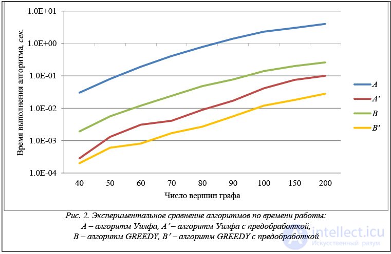
For the exact solution of MCP, Wilf's algorithm was used. This algorithm is recursive and finds an exact solution of MCP in time O(poly(n) ∙ 1.39n), where poly(n) – is some polynomial in n. In the two-phase procedure for solving MCP, the first phase (the MakeAtoms algorithm - decomposition of the graph into atoms) is performed in time O(n3), and the second phase (Wilf's algorithm for each atom and the linking of solutions) - in time O(n × poly(k) × 1.39k). Thus, the running time of the two-phase algorithm depends linearly on n = |V| and exponentially on the value k, tw(G) ≤ k. Thus, the more sparse the graph G is, the greater the effect achieved from its preprocessing when finding an exact solution of MCP with the aid of Wilf's algorithm.
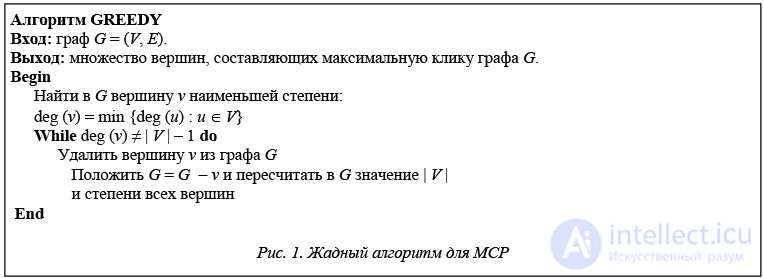
For solving the clique problem there also exists a large number of approximate solution algorithms, some of which are built on a greedy strategy. One such algorithm is given in figure 1. The running time of the GREEDY algorithm is O(n2). Application of this algorithm in the two-phase approach to solving the MCP problem for sparse graphs gives a running-time estimate of O(n ∙ k2).
Computational experiments carried out on random graphs confirmed the above-mentioned theoretical estimates of the running time of the two-phase algorithms and showed that they work significantly faster than the corresponding single-phase algorithms, and the order of the speedup substantially depends on the dimensionality and sparsity of the input graph (fig. 2).
Today, when the volumes of data being studied reach enormous sizes, algorithms and programs capable of processing these data in real time are in demand. The article considers a decomposition approach leading to a speedup of the operation of classical algorithms for solving
optimization problems on sparse graphs of large dimensionality. The approach is based on decomposing the original graph into atoms by clique minimal separators. The atomic representation of a graph can be created in advance in polynomial time and stored in the computer's external memory, and the atoms needed for processing can be successively loaded into main memory. The article presents algorithms and programs implementing the construction of such a representation. Further research on improving the considered decomposition approach is promising, aimed at accounting for possible changes over time in the composition of the vertices and edges of the original graph, and at applying it to routing problems in communication networks.

Comments