
Lecture
1. Loss system, example, characteristics
2 . Delay system (unlimited waiting or queue), example, characteristics
3. Mixed-type QS (with limited waiting
The complex nature of a market economy and the modern level of requirements it imposes
stimulate the use of more rigorous methods for analyzing its theoretical and practical problems. In recent decades mathematical methods have gained considerable
weight in economic research. Mathematical modeling is increasingly becoming one of the primary and most productive methods for studying economic processes and objects. Mathematical analysis of economic problems is organically
becoming part of economics. This positive assessment is also confirmed by the fact that
since 1969 the Nobel Prize in Economics has, as a rule, been awarded for
economic-mathematical research.
One of the important branches of economic-mathematical modeling is
queueing theory, which provides the theoretical foundations for the efficient design and operation of queueing systems. Queueing
systems (QS) are found in many areas of the economy (manufacturing, engineering,
the military sphere, everyday life, etc.) and are intended for repeated use in performing tasks of the same type.
Enormous resources are invested in the competition for customers in the modern economy. According to
estimates by Western economists, winning a new customer costs a firm six times more than retaining existing customers. And if a customer leaves dissatisfied,
winning them back requires spending 25 times more. In many cases customer dissatisfaction is caused by poor organization of service (too
long a wait in the queue, refusal of service, etc.). Using queueing
theory allows a firm to avoid such problems.
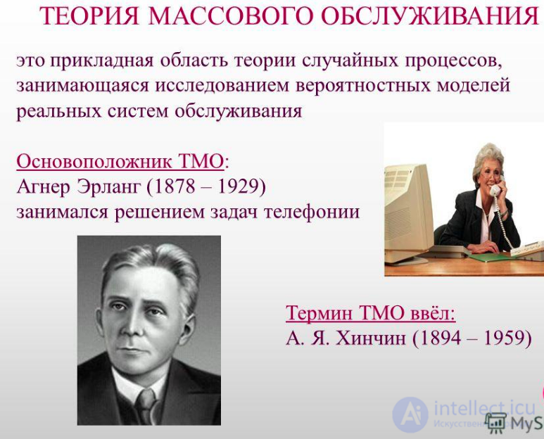
The founder of queueing theory is considered to be the Danish scientist A. K.
Erlang. As an employee of the Copenhagen Telephone Company, he published in 1909
a paper «The Theory of Probabilities and Telephone Conversations», in which he solved a number of problems in
the theory of loss systems.
A significant contribution to the creation and development of the general theory of queueing
was made by the outstanding Soviet mathematician Alexander Yakovlevich Khinchin (1984 – 1959), who proposed the very term queueing theory. In foreign literature the term
theory of queues is more often used.
In many areas of production, everyday services, economics and finance
systems1 of a special kind, implementing the repeated performance of
tasks of the same type, play an important role. Such systems are called queueing
systems (QS). Examples of QS in the financial and economic sphere include systems such as banks, insurance organizations, tax inspectorates, and audit services. In the sphere of production and services, examples of QS include: various communication systems (including telephone exchanges), loading and unloading complexes (ports, freight stations), gas stations, shops, hairdressing salons,
ticket offices, currency exchange points, repair shops, hospitals, etc. Systems such as computer networks, systems for collecting, storing and processing information, transport systems, automated production sites and, in the military sphere,
air defense or missile defense systems can also be regarded as
QS of a particular kind.
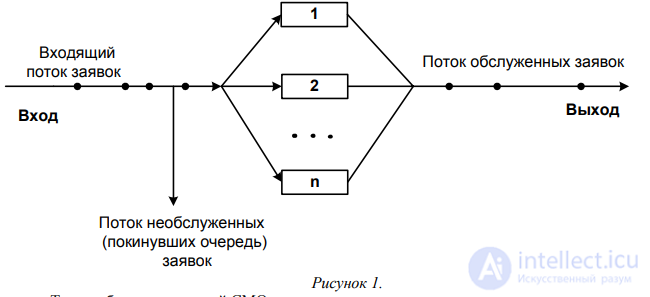
Diagram of a QS, fig. 1.
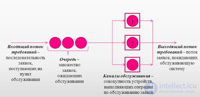
Every QS includes in its structure a certain number of service devices
(units, instruments, lines), which are called service channels. The role of channels can be
played by persons performing various operations (cashiers, operators, salespeople, hairdressers, etc.), communication lines, vehicles, cranes, repair crews, railway tracks, filling stations, etc.
Every QS is intended for servicing (performing) some flow of customers (or requests) arriving at the input of the system, for the most part not regularly, but at
random moments in time. Service of customers, in general, also takes not a constant, known in advance, but a random amount of time. After a customer has been served, the channel is freed and ready to accept the next customer. The random nature of the flow and of the service time leads to uneven loading of the QS: at some intervals of time
unserved customers may accumulate at the input of the QS (they either join the queue
or leave the QS unserved), while at other periods, with channels free, there will be
no customers at the input of the QS, which leads to underloading of the QS, i.e. to idle channels.
A diagram of the QS is shown in figure 1.
Thus, in any QS the following main elements can be identified:
1) the input flow of customers;
2) the queue;
3) the service channels;
4) the output flow of serviced customers.
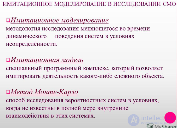
Depending on its parameters (the nature of the customer flow, the number of service channels and their productivity, as well as the rules governing the organization of work), every QS possesses a certain operating efficiency (throughput) that allows it to cope more or less successfully with the flow of customers.
Queueing theory studies QS.
The goal of queueing theory – the development of recommendations for the rational
design of a QS, the rational organization of its work, and the regulation of the flow of customers in order to
ensure a high operating efficiency of the QS.
To achieve this goal, the objectives of queueing theory are set, consisting in establishing the dependence of the operating efficiency of a QS on its organization (parameters): the nature of the customer flow, the number of channels and their productivity, and the rules
governing the operation of the QS.
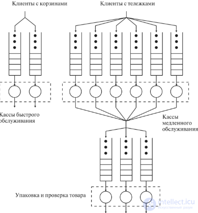
Fig. 15.3. Diagram of service in a supermarket
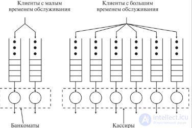
Fig. 15.2. Diagram of service in a bank

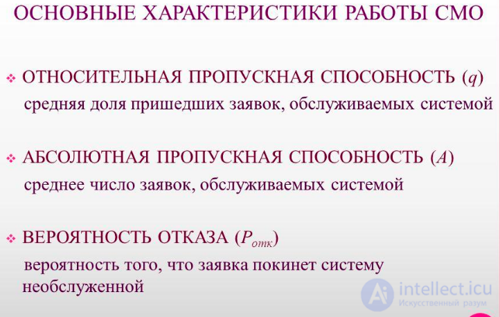
As characteristics of the operating efficiency of a QS one can choose
three main groups of (usually average) measures:
1. Measures of the effectiveness of QS utilization:
1.1. Absolute throughput of the QS – the average number of customers that the QS is able to serve per unit of time.
1.2. Relative throughput of the QS – the ratio of the average number of customers
served by the QS per unit of time to the average number of customers that arrived over the same
period of time.
1.3. The mean duration of the busy period of the QS.
1.4. Utilization factor of the QS – the mean proportion of time during which
the QS is occupied serving customers, etc.
2. Measures of the quality of customer service:
2.1. Mean waiting time of a customer in the queue.
2.2. Mean sojourn time of a customer in the QS.
2.3. Probability of a customer being refused service without waiting.
2.4. Probability that a newly arrived customer will be accepted for service immediately.
2.5. The distribution law of the waiting time of a customer in the queue.
2.6. The distribution law of the sojourn time of a customer in the QS.
2.7. Mean number of customers present in the queue.
2.8. Mean number of customers present in the QS, etc.
3. Measures of the operating effectiveness of the pair «QS – client», where by «client» is meant the entire set of customers or some source of them. Such measures include, for example, the mean income brought
by the QS per unit of time, etc.
The random nature of the customer flow and of the duration of their service gives rise, in
the QS, to a random process.
Definition. A random process (or random function) is a correspondence in which each value of the argument (in this case – a moment from the interval
of time over which the experiment is conducted) is made to correspond to a random variable (in this case
– the state of the QS).
Therefore, in order to solve the problems of queueing theory it is necessary to study
the random process taking place in the QS, i.e. it is necessary to construct and analyze
its mathematical model. The mathematical analysis of the operation of a QS is considerably simplified
if this random process satisfies certain conditions, which will be discussed below.
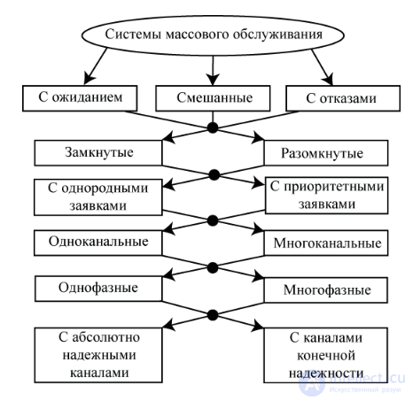
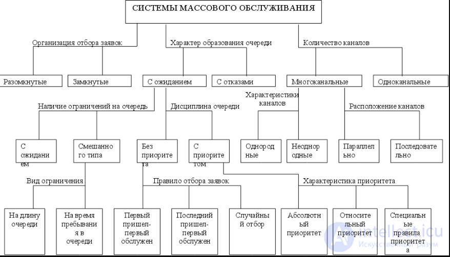
Queueing systems are divided into types (or classes) according to a number of features.
By the number of channels, QS are divided into single-channel (when there is one service
channel) and multichannel, or more precisely n-channel (when the number of channels n ≥ 2).
Here and below we shall assume that each channel can serve only
one customer at a time and, unless stated otherwise, each customer being served is served by only one channel. Multichannel QS can consist of homogeneous channels, or of heterogeneous ones differing in the duration of service of a single customer. In practice, the service time of a single customer by a channel Tserv is a continuous random variable. However, under the condition of absolute homogeneity of the arriving customers
and of the channels, the service time can also be a constant value (Tserv = const).

By service discipline, QS are divided into three classes:
1. Loss systems, in which a customer arriving at the input of the QS at a moment when all
channels are busy is given a «refusal» and leaves the QS («is lost»). For this customer to still
be served, it must arrive at the input of the QS again and be regarded in that case as
a customer arriving for the first time. An example of a loss system is the operation of an automatic telephone exchange: if
the dialed telephone number (the customer arriving at the input) is busy, the customer receives a refusal,
and to get through to that number one must dial it again (the customer arrives at the
input as a new one).
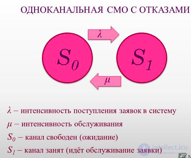
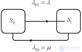
Figure 3. State transition diagram of a single-channel loss system.
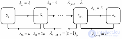
Figure 4. State transition diagram of a multichannel loss system.
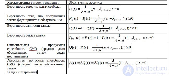
Characteristics of a single-channel loss system.
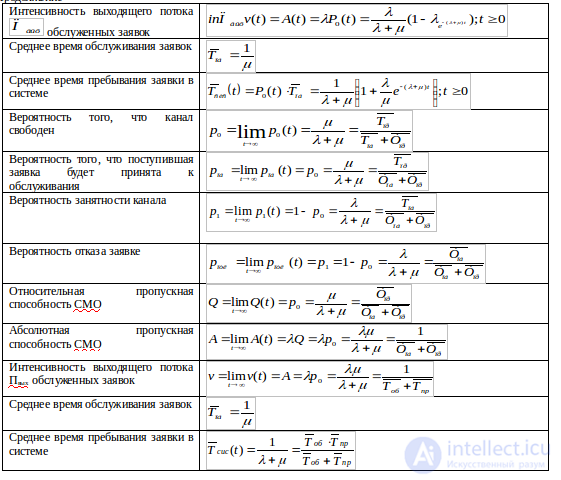
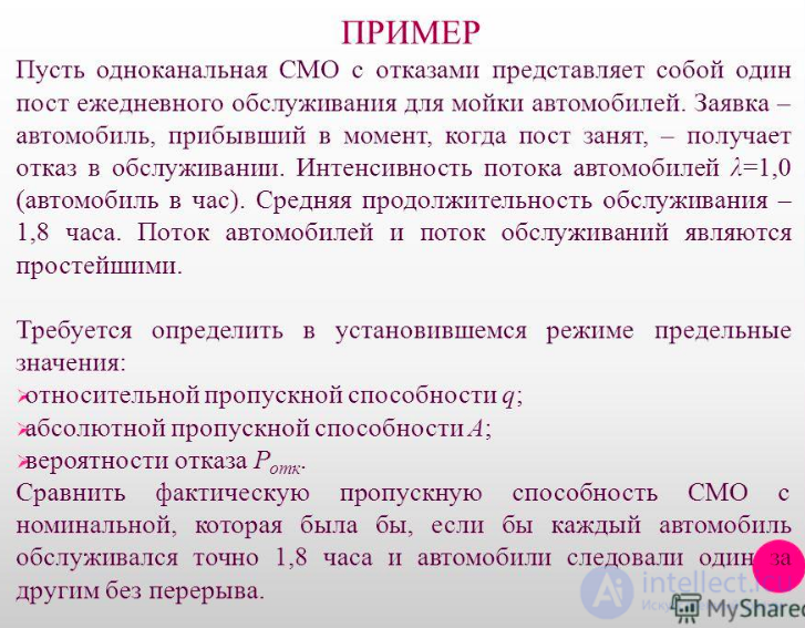
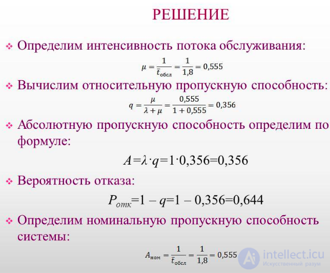
2. Delay system (unlimited waiting or queueing system). In such systems
a customer arriving at a moment when all channels are busy joins the queue and waits for a channel to become free, which will then accept it for service. Every customer arriving at the input
will eventually be served. Such QS are often found in retail trade, in the sphere of household and medical services, and at enterprises (for example, the servicing of machine tools by a crew of maintenance workers).

Figure 6. State transition diagram of a single-channel delay system.
The states of the QS have the following interpretation:
S0 - the channel is free;
S1 - the channel is busy (no queue);
S2 - the channel is busy (one customer is in the queue);
Sn - the channel is busy (n-1 customers are in the queue);
SN - the channel is busy (N-1 customers are in the queue).
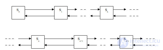
Figure 7. State transition diagram of a multichannel delay system.
Note that as the number of customers in the QS increases from 0 to n, the number of busy service channels increases. When the number of customers in the QS is greater than n, the service flow intensity remains equal to nµ.
Let us define the characteristics of a single-channel QSwith waiting and a finite queue length equal to (N —1):
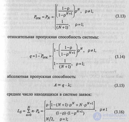

Let us consider an example of a single-channel delay system.
Example 3.2. A specialized diagnostic station is a single-channel QS. The number of parking spaces for cars waiting for diagnostics is limited and equal to 3 [(N- 1) = 3]. If all the parking spaces are occupied, i.e. three cars are already in the queue, then the next car arriving for diagnostics does not join the service queue. The flow of cars arriving for diagnostics is distributed according to the Poisson law and has an intensity l= 0.85 (cars per hour). The diagnostic time of a car is distributed according to the exponential law and is on average equal to 1.05 hours.
It is required to determine the probabilistic characteristics of the diagnostic station operating in the steady-state regime.
Solution
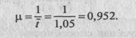
1. The parameter of the flow of car servicing:
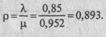
2. The traffic intensity of the flow of cars is determined as the ratio of the intensities l and m, i.e.
3. Let us calculate the limiting probabilities of the system:

P1=ρ·P0 = 0.893·0.248 = 0.221
P2=ρ2·P0 = 0.8932·0.248 = 0.198
P3=ρ3·P0 = 0.8933·0.248 = 0.177
P4=ρ4·P0 = 0.8932·0.248 = 0.158
4. The probability of a car being refused service:
Ploss=P4=ρ4·P0 ≈ 0.158
5. The relative throughput of the diagnostic station:
q=1-Ploss = 1-0.158 = 0.842
6. The absolute throughput of the diagnostic station
A=λ·q = 0.85·0.842 = 0.716 (cars per hour)
7. The mean number of cars being serviced and in the queue (i.e. in the queueing system):
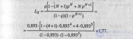
8. The mean sojourn time of a car in the system:

9. The mean duration of a customer's stay in the queue awaiting service:
Wq=WS-1/μ = 2.473-1/0.952 = 1.423 hours
10. The mean number of customers in the queue (queue length): Lq= A,(1 - PN) Wq= 0.85
Lq=λ(1-PN)·Wq = 0.85·(1-0.158)·1.423 = 1.02
The operation of the diagnostic station considered can be regarded as satisfactory, since the diagnostic station fails to service cars on average in 15.8% of cases (Ploss= 0.158).
3. Mixed-type QS (with limited waiting). These are systems in which certain restrictions are imposed on a customer's stay in the queue.
These restrictions may be imposed on the length of the queue, i.e. on the maximum possible
number of customers that can be in the queue at the same time. As an example of such
a system one can cite an automobile repair shop with a parking area of limited
size for faulty vehicles awaiting repair.
Waiting restrictions may concern the time a customer spends in the queue, after which it leaves the queue and leaves the system, or they may concern the total time
a customer spends in the QS (i.e. the combined time spent in the queue and under service).
In a delay system and in a mixed-type QS, various schemes for servicing customers from the queue are used. Service can be ordered, when customers from
the queue are served in the order of their arrival in the system, or unordered, in which customers from the queue are served in random order. Sometimes priority service is used, when certain customers from the queue are considered priority customers and are therefore served first.
By the restriction placed on the flow of customers, QS are divided into closed and open.
If the flow of customers is limited and customers that have left the system can return to it, then the QS is closed; otherwise it is – open. A classic example
of a closed QS is the work of a crew of maintenance workers in a workshop. The machines are the sources
of customers requiring service, and their number is limited; the maintenance workers – are the service channels.
After repair work has been carried out, a machine that has broken down again becomes a source of customers requiring service. In an open QS the characteristics of the customer flow do not depend on
the state of the QS itself (how many channels are busy). In a closed QS they – do depend on it.
Thus, in the example considered above, the intensity of the flow of «customers» from the machines (i.e.
the number of customers per unit of time) depends on how many of them are out of order and waiting for repair.
By the number of service stages, QS are divided into single-phase and multiphase
systems. If the channels of a QS are homogeneous, i.e. perform one and the same service operation, then such QS are called single-phase. If the service channels are arranged in sequence and are heterogeneous, since they perform different service operations
(i.e. service consists of several successive stages or phases), then the QS is called multiphase. An example of the operation of a multiphase QS is the servicing of cars at a vehicle service station (washing, diagnostics, etc.). Below we shall
consider only single-phase QS.
The structure of maximally efficient queues, and a look at the problem from the point of view of load balancing. What is load balancing? According to the definition from Wikipedia, it is: “…a methodology for distributing requests across several computers … that makes it possible to achieve optimal utilization of resources, maximize the throughput of the system, minimize the response time to a request, and avoid overload”
What is important here?
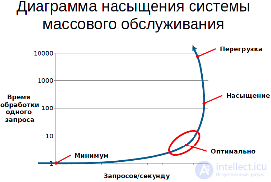
The graph – a saturation diagram. On one side, the number of requests per second, and on the other side – latency (in this context – the processing time of a single request).
The task, when we organize a queue, when we organize the processing of a queue – is to arrange things so that, on the one hand, we have a high utilization of resources, and on the other hand, we serve all customers with the maximum possible quality.
What does quality mean here? First and foremost, quality – is the processing time, the time spent waiting for a result. And if you look at a typical diagram of a system served by a queue – it looks exactly like this. That is, you can plot a graph of latency, and you can plot a graph of RPS. In terms of RPS, we may or may not notice a decrease in RPS. There are a large number of systems in which the number of requests per second decreases as the load increases.
What happens from the point of view of a queueing system? It performs useless work, i.e. at the moment of overload something happens that is not directed, one way or another, at the direct servicing of customers, but is instead directed at fighting the overload. For example, if we take a database, a typical example in a DB is a decrease in load, a decrease in performance as the number of transactions simultaneously present in the DB increases. This happens because there appears waiting on locks and on deadlocks’ occurrence. Waiting on a lock – is a useless thing to do; deadlocks’ overall effect, in general, is that transactions get restarted and have to be executed again – an example from a computer system.
In this situation we are interested in building a system that will stay in the optimal part of the curve, i.e. one that will handle the maximum possible number of requests while still preserving its performance characteristics.
In this sense you often come to realize that many people don't fully understand what they actually want, because latency and RPS – are unrelated things. That is, our desire to maximize the performance of the system and our desire to maximize the quality of service – are contradictory desires.
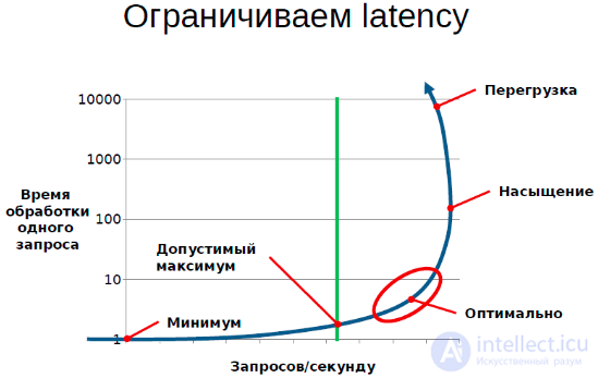
The graph shows qualitatively that if we want to limit latency specifically to a given value, then, at most, we can allow a certain load, and beyond that we cannot go, i.e. beyond that point the quality-of-service requirements effectively limit the throughput.
The second criterion by which we can optimize the system – is maximizing RPS.
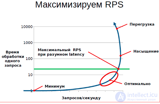
In this sense it is useful for us to reach some saturation point of the system, while maintaining a satisfactory level of service, and without moving into the overload region.
To understand why these are interrelated things, let me try to dig into queueing theory.
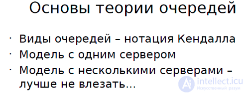
The single-server model – is fairly illustrative.
There are 2 ways to understand how a queueing system works:
If you try to dig into queueing theory, you come to realize that there can be a great many models.
Kendall's notation
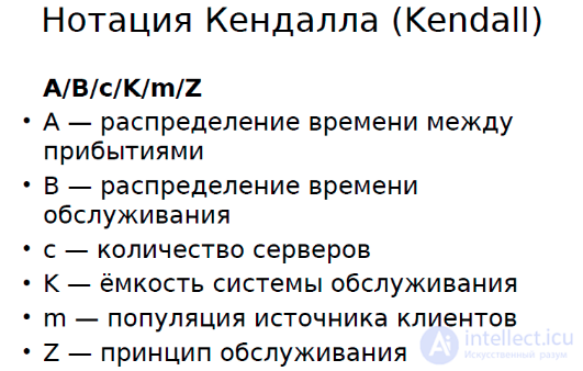
There is Kendall's notation – it classifies all systems by six indicators:
The simplest model that queueing theory gives – is the model for a single server.
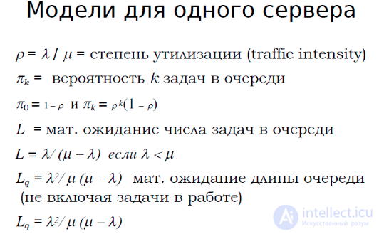
What do we get here? The degree of utilization – is the ratio of throughput to the rate (speed) of task arrivals. Suppose 1 server can handle 10 tasks per second, and 9 tasks per second arrive. It will probably cope with the load; on average, 9 – is the degree of utilization. Here it is worth saying – if the number of tasks per second exceeds the server's throughput, then it's game over, there is nothing special you can do about it, the queue will inevitably grow.
πk – is the probability of k tasks in the queue.
What is interesting here: suppose you have 10 tasks in the queue, the arrival rate of tasks – is 10 per second, and the server can handle 12 per second. What is the probability that, at the moment the next consumer arrives, the queue will be empty, i.e. that it will be able to receive service immediately? This is the probability that no one arrived before it – that is 2/12. With high probability, by the time the next task arrives, the server is already servicing some previous one, with probability 10/12, and with the complementary probability it is servicing no one – this is what the queueing theory model tells us. That is, if we want to maximize utilization, the queue will inevitably grow, because at the moment a new task arrives, the server is already busy servicing some other task, and the higher the utilization, the higher this probability. This is a basic insight of queueing theory.
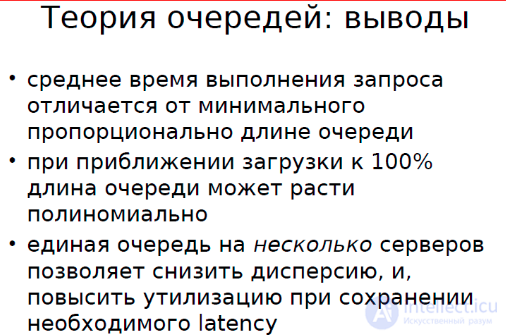
Here I am not giving models for several servers, but the basic idea is that if we have a single queue and multiple servers, then we can damp the dispersion in the distribution of participants by having all the servers receive a uniform load.
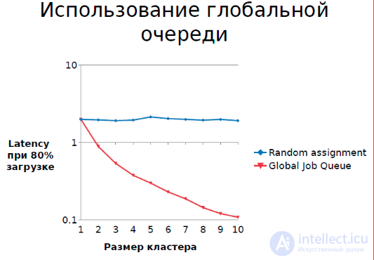
The result of a simulation where we have an 80% load on the cluster: the blue graph – is the case where a task arrives at a random server according to a random law, and the red graph – is the case where we have a global queue, and each server takes a task from the queue whenever it becomes available. As the number of servers increases, latency decreases – this is a real simulation.
1 – is the queue length in the case where, at 80% load, each server works independently. On average it has some queue. When it works from the global queue, the probability that at the moment of arrival there is no server available to perform the task – is within 0.1. Intuitively this makes sense: we have 10 workers and 8 tasks per worker at any given moment in time. The probability that a task has arrived and there is no free worker is small. If we have 10 workers and each one has its own task, then the probability increases.
What other insights can we take from queueing theory?
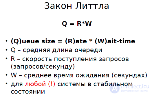
The general idea of Little's Law is that the number of tasks being served simultaneously is proportional to the service time and the arrival rate. What is important here in this case?
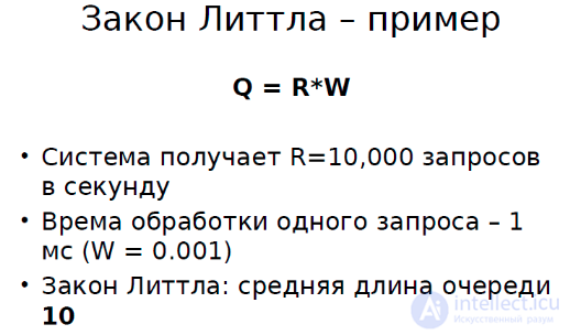
If your system receives 1000 requests per second, and the service time of one request – is 1 ms, then the average queue length in such a system will be 10 (the number of simultaneous tasks in the system). In general, if these are separate queues, i.e. if each worker has its own queue, then your average queue length can reach 10.
From the point of view of scaling, the conclusion from this is the following:
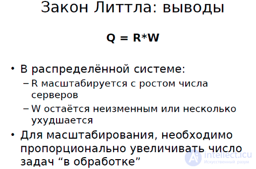
In order to grow proportionally, we need to scale the work more or less linearly, increasing the number of servers and the number of simultaneously served tasks. That is, if our task is large, then increasing the number of servers is not guaranteed to increase our performance. And because we have to increase the number of servers, the total number of tasks in flight grows, and accordingly the time spent on all sorts of warm-ups, the cost of idle time, etc., etc. also grows.
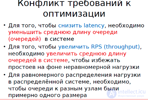
Conclusion: we have a conflict of requirements, and in order to satisfy it, we need to reduce the load on the system in one way or another. This is the main conclusion that the theory gives us.

Comments