Queueing Systems: Concept, Principle of Operation, Examples, Analysis and Synthesis

A large class of systems that are difficult to study by analytical methods, but that are well studied by methods of statistical modeling, can be reduced to queueing systems (QS).

The concept of a QS

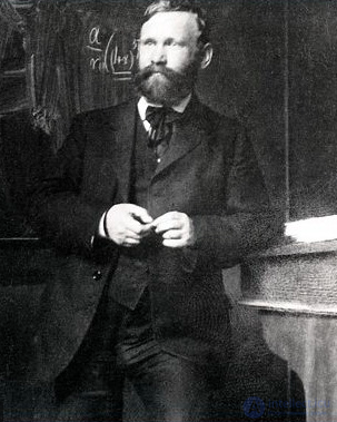
The founder of queueing theory was the Danish scientist A.K. Erlang
• 1909 «The Theory of Probabilities and Telephone Conversations»
The term queueing theory was proposed by A.Ya. Khinchin
• 1932 «Mathematical Theory of a Stationary Queue»
• 1933 «On the Average Idle Time of Machines»
• 1963 «Works on the Mathematical Theory of Queueing»
In foreign literature the term queueing theory is used more often

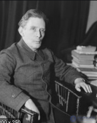
Aleksandr Yakovlevich Khinchin

Queueing systems – are systems in which service requests arrive at random moments in time, and
the arriving requests are served using the service channels available to the system.

The goal of queueing theory is to develop recommendations for the rational design of a QS, the rational organization
of its operation, and the regulation of the flow of requests to ensure a high efficiency of QS functioning.

A queueing system (QS) — is a system that services requests arriving into it. The servicing of requests in a QS is carried out by service units. A classical QS contains from one to an infinite number of units. Depending on whether arriving requests have the possibility of waiting for service to begin, QSs are divided into:

• loss systems, in which requests that do not find a single free unit at the moment of arrival are lost;
• waiting systems, in which there is a buffer of infinite capacity for buffering arriving requests, with waiting requests forming a queue;
• systems with a finite-capacity buffer (waiting with limitations), in which the queue length cannot exceed the buffer capacity; here a request arriving at an overflowing QS (no free waiting positions available) is lost.

The selection of a request from the queue for service is carried out using a so-called queueing discipline. Examples of these are FCFS/FIFO (the first to arrive is served first), LCFS/LIFO (the last to arrive is served first), and random (random selection). In waiting systems the buffer can in general have a complex structure.

How a QS works

Examples of QS

• Customer service in retail trade
• Transport service
• Medical service of the population
• Repair of equipment, machines, and mechanisms in operation
• Processing of documents in a management system
• Tourist services

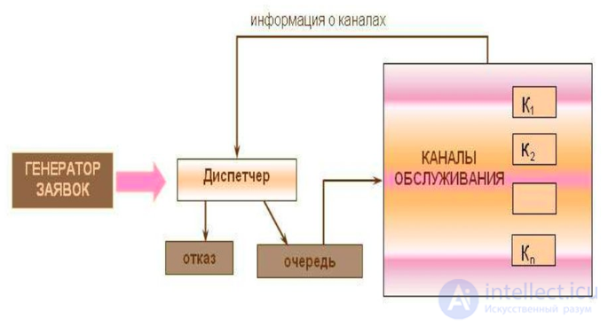
A QS assumes that there are typical paths (service channels) through which requests pass in the course of processing. It is customary to say that requests are serviced by channels. Channels can differ in purpose and characteristics, and they can be combined in different combinations; requests may stand in queues and wait for service. Some requests may be serviced by channels, while others may be denied service. It is important that, from the system's point of view, requests are abstract: they are something that wishes to be serviced, that is, to pass through a certain path in the system. Channels are also an abstraction: they are what services requests.

Requests can arrive unevenly, channels can service different requests in different amounts of time, and so on, and the number of requests is always quite large. All this makes such systems difficult to study and manage, and it is not possible to trace all the cause-and-effect relationships in them. Therefore it is customary to view servicing in complex systems as random in nature.

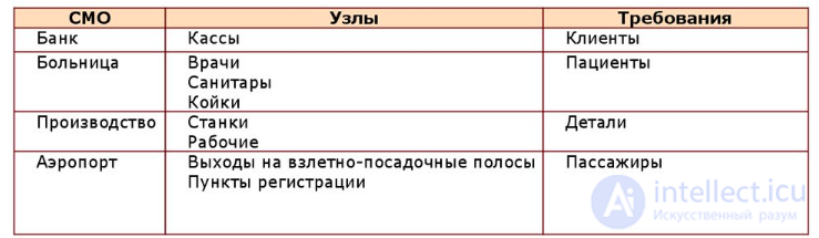
Examples of a QS (see Table 30.1) can include: a bus route and passenger transportation; a production conveyor for processing parts; a squadron of aircraft flying into foreign territory, which is «serviced» by anti-aircraft defense guns; the barrel and magazine of a submachine gun, which «service» cartridges; electric charges moving in some device, etc.

Table 30.1. Examples of queueing systems

But all these systems are combined into a single class of QS, since the approach to studying them is the same. It consists in the fact that, first, random numbers are generated using a random number generator, which simulate the RANDOM moments at which requests appear and the time of their service in channels. But taken together these random numbers are, of course, subject to statistical regularities.

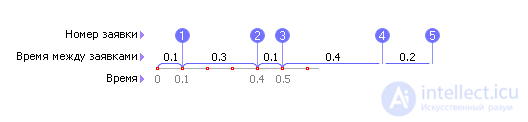
For example, suppose it is said: «requests arrive on average in a quantity of 5 per hour». This means that the times between the arrival of two neighboring requests are random, for example: 0.1; 0.3; 0.1; 0.4; 0.2, as shown in Fig. 30.1, but on average they add up to 1 (note that in the example this is not exactly 1, but 1.1 — but in another hour this sum, for example, may equal 0.9); and only over a sufficiently long time will the average of these numbers become close to one hour.

Fig. 30.1. Random process of request arrivals in a QS

The result (for example, the throughput of the system), of course, will also be a random variable over individual time intervals. But when measured over a large time interval, this value will, on average, already correspond to the exact solution. That is, for characterizing a QS, one is interested in answers in a statistical sense.

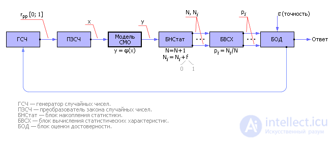
So, the system is tested with random input signals subject to a given statistical law, and statistical indicators, averaged over the observation time or over the number of trials, are taken as the result. Earlier, in Lecture 21 (see Fig. 21.1), we already developed a scheme for such a statistical experiment (see Fig. 30.2).

Fig. 30.2. Scheme of a statistical experiment for studying queueing systems

Second, all QS models are assembled in a typical way from a small set of elements (channel, request source, queue, request, queueing discipline, stack, ring, and so on), which makes it possible to simulate these problems in a typical way. To do this, the system model is assembled from a construction set of such elements. It does not matter which specific system is being studied; what matters is that the system's scheme is assembled from the same elements. Of course, the structure of the scheme will always be different.

Let us list some basic concepts of a QS.

• Request (customer) — a request for service.
• Input flow of requests — the totality of requests arriving into the QS.
• Service time — the period of time during which a request is serviced.
• Mathematical model of a QS — this is a set of mathematical expressions describing the input flow of requests, the service process, and their interrelation.

Channels — that which services; there are hot ones (they start servicing a request the moment it arrives at the channel) and cold ones (the channel needs time to prepare before it can start servicing). Request sources — generate requests at random moments in time, according to a statistical law given by the user. Requests, also called customers, enter the system (are generated by request sources), pass through its elements (are serviced), and leave it either serviced or unsatisfied. There are impatient requests — those that get tired of waiting or of being in the system and leave the QS of their own accord. Requests form flows — the flow of requests at the input of the system, the flow of serviced requests, the flow of rejected requests. A flow is characterized by the number of requests of a certain kind observed at some point of the QS per unit of time (hour, day, month), that is, a flow is a statistical quantity.

Queues are characterized by the rules for standing in the queue (the queueing discipline), the number of places in the queue (the maximum number of customers that can be in the queue), and the structure of the queue (the relationship between places in the queue). There are finite and infinite queues. Let us list the most important queueing disciplines. FIFO (First In, First Out — first come, first served): if a request arrived in the queue first, it will be the first to go to service. LIFO (Last In, First Out — last come, first served): if a request arrived in the queue last, it will be the first to go to service (example — cartridges in a submachine gun's magazine). SF (Short Forward — short jobs forward): requests from the queue that have a shorter service time are serviced first.

Let us give a vivid example showing how the correct choice of one or another queueing discipline can yield a tangible saving of time.

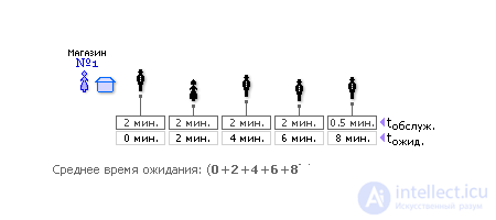
Suppose there are two stores. In store No. 1 service is carried out in queue order, that is, the FIFO queueing discipline is implemented here (see Fig. 30.3).

Fig. 30.3. Organizing a queue under the FIFO discipline

The service time t_serv in Fig. 30.3 shows how much time the salesperson will spend servicing one customer. It is clear that when buying an individually-packaged item, the salesperson will spend less time on service than when buying, say, bulk products requiring additional manipulations (scooping, weighing, calculating the price, etc.). The waiting time W_q shows how much time will pass before the next customer in line is serviced by the salesperson.

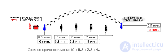
In store No. 2 the SF discipline is implemented (see Fig. 30.4), meaning that an individually-packaged item can be bought out of turn, since the service time t_serv for such a purchase is small.

Fig. 30.4. Organizing a queue under the SF discipline

As can be seen from both figures, the last (fifth) customer is about to buy an individually-packaged item, so his service time is small — 0.5 minutes. If this customer comes to store No. 1, he will be forced to stand in the queue for a full 8 minutes, whereas in store No. 2 he will be served immediately, out of turn. Thus, the average service time for each customer in the store with the FIFO queueing discipline will be 4 minutes, while in the store with the SF discipline — only 2.8 minutes. And the social benefit, the time saved, will amount to: (1 – 2.8/4) · 100% = 30 percent! So, 30% of the time saved for society — and this is achieved solely through the correct choice of queueing discipline.

A systems specialist must have a good understanding of the performance and efficiency resources of the systems he designs, hidden in the optimization of parameters, structures, and queueing disciplines. Modeling helps to reveal these hidden reserves.

When analyzing modeling results, it is also important to indicate the interests involved and the degree to which they are satisfied. A distinction is made between the interests of the customer and the interests of the owner of the system. Note that these interests do not always coincide.

The performance of a QS can be judged by performance measures. The most popular of these are:

• probability of service of a customer by the system;
• throughput of the system;
• probability of denial of service to a customer;
• probability that each individual channel is busy and that all of them are busy together;
• mean busy time of each channel;
• probability that all channels are busy;
• mean number of busy channels;
• probability of idleness of each channel;
• probability of idleness of the entire system;
• mean number of requests standing in the queue;
• mean waiting time of a request in the queue;
• mean service time of a request;
• mean time a request spends in the system.

The quality of the resulting system should be judged from the totality of the values of the performance measures. When analyzing modeling results (performance measures), it is also important to pay attention to the interests of the customer and the interests of the owner of the system, that is, whether this or that measure should be minimized or maximized, as well as the degree to which they are satisfied. Note that most often the interests of the customer and the owner do not coincide with each other, or do not always coincide. We will hereafter denote the performance measures by H = {h₁, h₂, …}.

The parameters of a QS can be: the arrival rate of the flow of requests, the service rate of the flow of service, the average time during which a request is willing to wait for service in the queue, the number of service channels, the queueing discipline, and so on. Parameters — are what affects the performance measures of the system. We will hereafter denote parameters as R = {r₁, r₂, …}.

Example. A gas station (filling station).

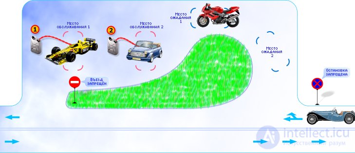
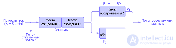
1. Problem statement. Fig. 30.5 shows the layout of the filling station. Let us consider the method of modeling a QS using this as an example, and the plan for studying it. Drivers passing along the road by the filling station may want to fill up their car. Not all motorists in the flow want to be serviced (fill the car with gasoline); suppose that out of the whole flow of cars, on average 5 cars per hour pull in for fuel.

Fig. 30.5. Layout of the filling station being modeled

The filling station has two identical pumps, the statistical throughput of each of which is known. The first pump on average services 1 car per hour, the second on average — 3 cars per hour. The owner of the filling station has paved a place for cars where they can wait for service. If the pumps are occupied, other cars can wait for service in this place, but no more than two at a time. We will consider the queue to be common to both pumps. As soon as one of the pumps becomes free, the first car in the queue can take its place at the pump (with the second car then moving up to the first place in the queue). If a third car appears while all the places (there are two) in the queue are occupied, it is denied service, since it is forbidden to stand on the road (see the road signs near the filling station). Such a car drives away from the system forever and, as a potential customer, is lost to the owner of the filling station. The problem could be made more complex by considering a cash register (another service channel that must be visited after service at one of the pumps) and the queue to it, and so on. But in the simplest version it is obvious that the paths of the flows of requests through the QS can be depicted as an equivalent diagram, and by adding the values and notation of the characteristics of each element of the QS, we finally obtain the diagram shown in Fig. 30.6.

Fig. 30.6. Equivalent diagram of the modeling object

2. Method for studying a QS. In our example we will apply the principle of sequential tracing of requests (for details on modeling principles, see Lecture 32). Its idea is that a request is traced through the entire system from input to output, and only after that does one proceed to model the next request.

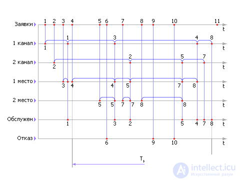
For clarity, let us build a timing diagram of the QS's operation, showing on each timeline (the time axis t) the state of an individual element of the system. As many timelines are drawn as there are different places, flows, in the QS. In our example there are 7 of them (the flow of requests, the flow of waiting in the first place in the queue, the flow of waiting in the second place in the queue, the flow of service in channel 1, the flow of service in channel 2, the flow of requests serviced by the system, the flow of denied requests).

To generate the arrival time of requests we use the formula for calculating the interval between the moments of arrival of two random events (see Lecture 28):

In this formula the flow value λ must be given (before this it must be determined experimentally on the object as a statistical average), and r — is a random uniformly distributed number from 0 to 1 from an RNG or a table, in which the random numbers should be taken in sequence (without selecting them specially).

Problem. Generate a flow of 10 random events with an event occurrence rate of 5 units/hour.

Solution of the problem. Let us take random numbers uniformly distributed on the interval from 0 to 1 (see the table), and calculate their natural logarithms (see Table 30.2).

The formula for a Poisson flow defines the distance between two random events as follows: t = –Ln(r_u)/λ. Then, given that λ = 5, we have the distances between two neighboring random events: 0.68, 0.21, 0.31, 0.12 hours. That is, the events occur: the first — at the moment t = 0, the second — at the moment t = 0.68, the third — at the moment t = 0.89, the fourth — at the moment t = 1.20, the fifth — at the moment t = 1.32, and so on. Let us plot the events, the arrival of requests, — on the first timeline (see Fig. 30.7).

Fig. 30.7. Timing diagram of the QS's operation

The first request is taken and, since the channels are free at this moment, it is placed into service in the first channel. Request 1 is transferred to the «channel 1» timeline.

The service time in a channel is also random and is calculated by an analogous formula:

where the role of the rate is played by the service flow value μ₁ or μ₂, depending on which channel is servicing the request. We find on the diagram the moment when service ends, by laying off the generated service time from the moment service began, and we drop the request onto the «Serviced» timeline.

The request has passed through the entire path in the QS. Now, following the principle of sequential tracing of requests, we can also simulate the path of the second request.

If at some moment it turns out that both channels are occupied, the request should be placed in the queue. In Fig. 30.7 this is request number 3. Note that, under the conditions of the problem, unlike in the channels, requests do not spend a random time in the queue but instead wait until one of the channels becomes free. After a channel becomes free, the request moves up to the timeline of the corresponding channel and is serviced there.

If all the places in the queue are occupied at the moment the next request arrives, the request should be sent to the «Denied» timeline. In Fig. 30.7 this is request number 6.

The procedure of simulating the servicing of requests is continued for some observation time T_obs. The longer this time, the more accurate the modeling results will subsequently be. In practice, for simple systems T_obs is chosen equal to 50—100 hours or more, although sometimes it is better to measure this quantity by the number of requests considered.

Analysis of the timing diagram

We will carry out the analysis on the example already considered.

First we need to wait for the steady-state regime to be established. We discard the first four requests as atypical, occurring during the process of the system's operation settling in. We measure the observation time; suppose that in our example it amounts to T_obs = 5 hours. From the diagram we count the number of serviced requests N_serv, the idle times, and other quantities. As a result we can calculate the performance measures characterizing the quality of the QS's operation.

1. Probability of service: P_serv = N_serv/N = 5/7 = 0.714. To calculate the probability of service of a request in the system, it is enough to divide the number of requests that managed to be serviced during the time T_obs (see the «Serviced» timeline) N_serv, by the number of requests N that wanted to be serviced during this same time. As before, we determine the probability experimentally as the ratio of events that occurred to the total number of events that could have occurred!
2. Throughput of the system: A = N_serv/T_obs = 7/5 = 1.4 [units/hour]. To calculate the throughput of the system, it is enough to divide the number of serviced requests N_serv by the time T_obs during which this servicing took place (see the «Serviced» timeline).
3. Probability of loss: P_loss = N_loss/N = 3/7 = 0.43. To calculate the probability of a request being denied service, it is enough to divide the number of requests N_loss that were denied during the time T_obs (see the «Denied» timeline), by the number of requests N that wanted to be serviced during this same time, that is, that arrived into the system. Note. P_loss + P_serv should theoretically equal 1. In reality, the experimental result was P_loss + P_serv = 0.714 + 0.43 = 1.144. This inaccuracy is explained by the fact that the observation time T_obs is short and the statistics accumulated are insufficient to obtain a precise answer. The error of this measure is currently 14%!
4. Probability that one channel is busy: P₁ = T_busy/T_obs = 0.05/5 = 0.01, where T_busy — the time during which only one channel (the first or the second) is busy. The time intervals in which certain events occur are subject to measurement. For example, on the diagram we look for the intervals during which either the first or the second channel is busy. In this example there is one such interval at the end of the diagram, 0.05 hours long. The share of this interval in the total observation time (T_obs = 5 hours) is found by division and gives the sought probability of being busy.
5. Probability that both channels are busy: P₂ = T_busy/T_obs = 4.95/5 = 0.99. On the diagram we look for the intervals during which both the first and the second channel are busy at the same time. In this example there are four such intervals, and their sum is 4.95 hours. The share of the duration of this event in the total observation time (T_obs = 5 hours) is found by division and gives the sought probability of being busy.
6. Mean number of busy channels: n_busy = 0 · P₀ + 1 · P₁ + 2 · P₂ = 0.01 + 2 · 0.99 = 1.99. To calculate how many channels are busy in the system on average, it is enough to know the share (probability that one channel is busy) and multiply it by the weight of that share (one channel), know the share (probability that two channels are busy) and multiply it by the weight of that share (two channels), and so on. The resulting figure of 1.99 shows that, out of the two available channels, on average 1.99 channels are loaded. This is a high load indicator, 99.5%, meaning the system uses the resource well.
7. Probability that at least one channel is idle: P^*₁ = T_idle1/T_obs = 0.05/5 = 0.01.
8. Probability that both channels are idle at the same time: P^*₂ = T_idle2/T_obs = 0.
9. Probability that the whole system is idle: P^*_sys = T_{idle sys.}/T_obs = 0.
10. Mean number of customers in the queue: L_q = 0 · P_0q + 1 · P_1q + 2 · P_2q = 0.34 + 2 · 0.64 = 1.62 [units]. To determine the mean number of customers in the queue, it is necessary to determine separately the probability that there is one customer in the queue P_1q, the probability that there are two customers in the queue P_2q, and so on, and again add them up with the corresponding weights.
11. Probability that there is one customer in the queue: P_1q = T_1q/T_obs = 1.7/5 = 0.34 (there are four such intervals on the diagram in total, giving a sum of 1.7 hours).
12. Probability that there are two customers in the queue at the same time: P_2q = T_2q/T_obs = 3.2/5 = 0.64 (there are three such intervals on the diagram in total, giving a sum of 3.25 hours).
13. Mean waiting time of a customer in the queue:

    

    (Add up all the time intervals during which some customer was in the queue, and divide by the number of customers). There are 4 such customers on the time diagram.
14. Mean service time of a customer:

    

    (Add up all the time intervals during which some customer was being served at some channel, and divide by the number of customers).
15. Mean time a customer spends in the system: T_{avg. sys.} = T_{avg. wait.} + T_{avg. serv.}.
16. Mean number of customers in the system:

    

    Let us divide the observation interval, for example, into ten-minute segments. Over five hours this gives K subintervals (in our case K = 30). In each subinterval we determine from the time diagram how many customers are in the system at that moment. We need to look at rows 2, 3, 4 and 5 — which of them are busy at the given moment. Then the sum of the K terms is averaged.

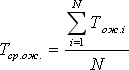
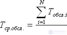
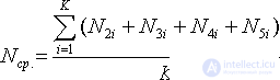
Next, the accuracy of each of the obtained results should be assessed. That is, we must answer the question: how much can we trust these values? The accuracy assessment is carried out using the method described in Lecture 34.

If the accuracy is not satisfactory, the duration of the experiment should be increased, thereby improving the statistics. It can also be done differently. Run the experiment several times again for a duration T_obs. Afterwards, average the values of these experiments. And check the results against the accuracy criterion again. This procedure should be repeated until the required accuracy is achieved.

Next, a table of results should be drawn up and the value of each of them should be assessed from the point of view of the customer and the owner of the QS (see Table 30.3).. In conclusion, taking into account what was said in each point, a general conclusion should be drawn. The table should look approximately as shown in Table 30.3.

Synthesis of a QS

We have carried out the analysis of the existing system. This has made it possible to see its shortcomings and to determine directions for improving its quality. But the answers to specific questions remain unclear: what exactly needs to be done — increase the number of channels, or increase their throughput, or increase the number of places in the queue, and, if increased, by how much? There are also questions such as which is better — to create 3 channels with a capacity of 5 units/hour or one with a capacity of 15 units/hour?

To assess the sensitivity of each measure to a change in the value of a given parameter, one proceeds as follows. All parameters except the chosen one are fixed. Then the values of all measures are recorded for several values of this chosen parameter. Of course, the simulation procedure has to be repeated again and again, and the measures averaged for each value of the parameter, and the accuracy assessed. But as a result, reliable statistical dependences of the characteristics (measures) on the parameter are obtained.

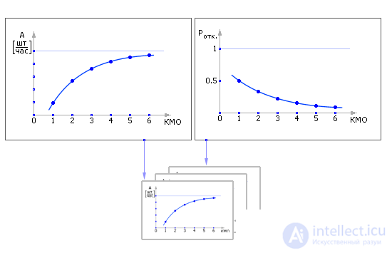
For example, for the 12 measures in our example, 12 dependences on a single parameter can be obtained: the dependence of the loss probability P_loss. on the number of places in the queue (NPQ), the dependence of the throughput A on the number of places in the queue, and so on (see Fig. 30.8).

Fig. 30.8. An approximate view of the dependence of measures on QS parameters

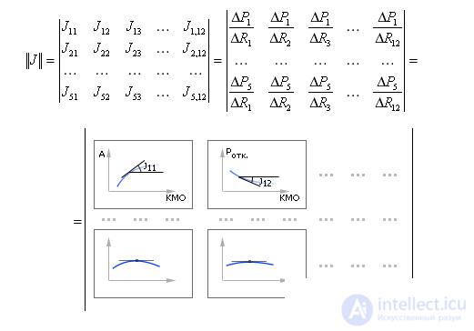
Then, in the same way, another 12 dependences of the measures P on another parameter R, having fixed the other parameters. And so on. This forms a kind of matrix of dependences of the measures P on the parameters R, which can be used for further analysis of the prospects of moving (improving the measures) in one direction or another. The slope of the curves shows the sensitivity well, i.e. the effect of moving along a given measure. In mathematics this matrix is called the Jacobian J, in which the role of the slope of the curves is played by the values of the derivatives ΔP_i/ΔR_j, see Fig. 30.9. (Recall that the derivative is geometrically related to the angle of inclination of the tangent to the dependence.)

Fig. 30.9. The Jacobian — a matrix of the sensitivities of the measures depending on changes in QS parameters

If there are 12 measures and, say, 5 parameters, then the matrix has dimension 12 x 5. Each element of the matrix — a curve, the dependence of the i-th measure on the j-th parameter. Each point of the curve — the mean value of the measure over a sufficiently representative interval T_obs, or averaged over several experiments.

It should be understood that the curves were recorded under the assumption that all parameters except one remained unchanged while they were being recorded. (If all the parameters were to change their values, the curves would be different. But this is not done, since it would result in complete confusion and the dependences would not be visible.)

Therefore, if, based on a review of the recorded curves, a decision is made that some parameter in the QS will be changed, then all the curves for the new point, at which the question of which parameter should be changed in order to improve the measures will again be investigated, should be recorded anew.

In this way, step by step, one can try to improve the quality of the system. But so far this method cannot answer a number of questions. The fact is that, first, if the curves increase monotonically, the question arises of where exactly one should stop. Second, contradictions can arise: one measure may improve when a chosen parameter is changed, while another may simultaneously worsen. Third, a number of parameters are difficult to express numerically, for example, a change in the queueing discipline, a change in the directions of the flows, a change in the topology of the QS. In the latter two cases, the search for a solution is carried out using expert assessment methods (see Lecture 36. Expert assessment) and artificial intelligence methods (see genetic algorithms in artificial intelligence.

Therefore, for now we will discuss only the first question. How should one decide what the value of the parameter should ultimately be, if the measure keeps improving monotonically as it increases? An infinite value is unlikely to satisfy an engineer.

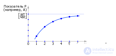
The parameter R — the control, is what is at the disposal of the QS owner (for example, the possibility of paving the site and thereby increasing the number of places in the queue, adding extra channels, increasing the arrival flow by increasing advertising expenses, and so on). By changing the control, one can influence the value of the measure P, the goal, the criterion (loss probability, throughput, mean service time, and so on). From Fig. 30.10 it can be seen that if the control R is increased, an improvement in the measure P can always be achieved. But it is obvious that any control is associated with costs Z. And the more effort is applied to control, the greater the value of the control parameter, the greater the costs. Usually the cost of control grows linearly: Z = C₁ · R. Although there are cases where, for example, in hierarchical systems, they grow exponentially, sometimes — inversely exponentially (bulk discounts), and so on.

Fig. 30.10. Dependence of the measure P on the controlled parameter R (example)

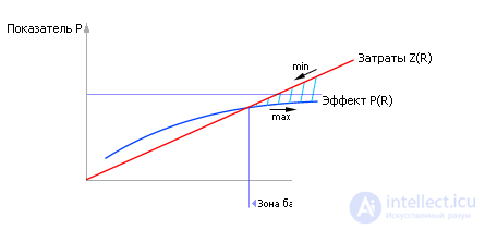
In any case, it is clear that at some point investing in more and more costs simply stops paying off. For example, the effect of paving a site of 1 km² is unlikely to pay back the costs of the owner of a gas station in Uryupinsk — there simply won't be that many people wanting to fill up on gasoline. In other words, the measure P in complex systems cannot grow indefinitely. Sooner or later its growth slows down. But the costs Z keep growing (see Fig. 30.11).

Fig. 30.11. Dependences of the effect of applying the measure P and the cost Z of obtaining it, as functions of the controlled parameter R

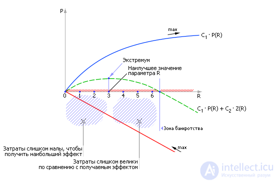
From Fig. 30.11 it can be seen that, by assigning a price C₁ per unit of cost R and a price C₂ per unit of the measure P, these curves can be added together. Curves are added if they need to be minimized or maximized simultaneously. If one curve is to be maximized and the other minimized, then their difference should be found, for example point by point. Then the resulting curve (see Fig. 30.12), which takes into account both the effect of the control and the cost of achieving it, will have an extremum. The value of the parameter R that provides the extremum of the function is precisely the solution of the synthesis problem.

Fig. 30.12. Combined dependence of the effect of applying the measure P and the cost Z of obtaining it, as functions of the controlled parameter R

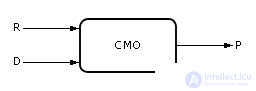
Besides the control R and the measure P, a disturbance also acts in systems. Let us denote disturbances as D = {d₁, d₂, …}, see Fig. 30.13. A disturbance is an input effect which, unlike a control parameter, does not depend on the will of the system owner. For example, low outdoor temperatures and competition unfortunately reduce the flow of customers, and equipment breakdowns annoyingly reduce the performance of the system. And the system owner cannot directly control these quantities. Usually the disturbance acts «to spite» the owner, reducing the effect P from the control efforts R. This happens because, in general, a system is created to achieve goals that are unattainable by themselves in nature. A person, by organizing a system, always hopes to use it to achieve some goal P. To this end, they expend effort R, going against nature. A system — the organization of nature's components, accessible to and studied by a person, in order to achieve some new goal that was previously unattainable by other means.

Fig. 30.13. Conventional notation for the system under study, acted upon by the control actions R and the disturbances D

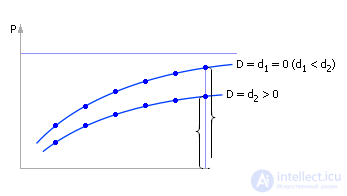
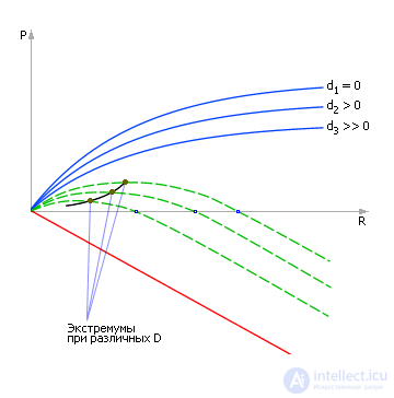
So, if we record the dependence of the measure P on the control R once again (as shown in Fig. 30.10), but under conditions of an emerged disturbance D, the shape of the curve may change. Most likely, for the same values of the controls, the measure will be lower, since the disturbance has a «spiteful» character, reducing the system's measures (see Fig. 30.14). A system left to itself, without efforts of a controlling nature, stops ensuring the goal for which it was created. If, as before, we plot the cost dependence and relate it to the dependence of the measure on the control parameter, the extremum point found will shift (see Fig. 30.15) compared to the case «disturbance = 0» (see Fig. 30.12).

Fig. 30.14. Dependence of the measure P on the control parameter R for various values of the disturbances D acting on the system

If the disturbance is increased again, the curves will change (see Fig. 30.14) and, as a result, the position of the extremum point will change again (see Fig. 30.15).

Fig. 30.15. Finding the extremum point on the combined dependence for various values of the acting disturbance factor D

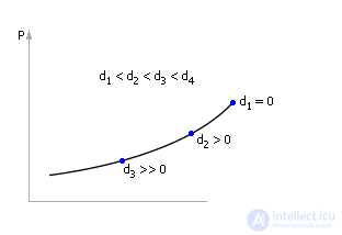
Ultimately, all the found positions of the extremum points are transferred to a new graph, where they form the dependence of the Measure P on the Control parameter R as the Disturbances D change (see Fig. 30.16).

Fig. 30.16. Dependence of the measure P on the control parameter R as the values of the disturbances D change (the curve consists only of extremum points)

Note that in reality there may also be other operating points on this graph (the graph is, as it were, permeated by families of curves), but the points we have plotted set such coordinates of the control parameter at which, for the given disturbances (!), the highest possible value of the measure P is achieved.

This graph (see Fig. 30.16) links the Measure P, the Control (resource) R, and the Disturbance D in complex systems, indicating how the DM (decision maker) should act in the best way under the disturbances that have arisen. Now, knowing the actual situation at the facility (the value of the disturbance), the user can quickly use the graph to determine what control action on the facility is needed to ensure the best value of the measure of interest to them.

Note that if the control action is less than optimal, the overall effect will decrease, resulting in a situation of lost profit. If the control action is greater than optimal, the effect will also decrease, since the price to be paid for a further increase in control effort will be greater in magnitude than what you will gain from using it (a situation of bankruptcy).

Note. In the text of the lecture we used the words «control» and «resource», that is, we assumed that R = U. It should be explained that control indeed plays the role of a certain limited value for the owner of the system. That is, it is always a valuable resource for them, one that always has to be paid for and is always in short supply. Indeed, if this quantity were not limited, we could achieve infinitely large values of the goals through an infinitely large amount of control, but infinitely large results are clearly not observed in nature.

Sometimes control proper U is distinguished from the resource R, calling the resource a certain reserve, that is, the boundary of the possible value of the control action. In this case the concepts of resource and control do not coincide: U < R. Sometimes a distinction is made between the limiting value of control U ≤ R and the integral resource ∫Udt ≤ R.

See also

• [[b7519]]

See also

• 19.1. The subject of queuing theory