
Lecture 19 min.
Definition: The logarithm of a positive number b to the base  is the exponent c to which the number a must be raised to obtain the number b.
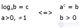
The basic logarithmic identity:
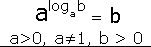
Properties of logarithms:
The basic logarithmic identity
The basic logarithmic identity follows from the definition of the logarithm[7]:

Corollary: if two real logarithms are equal, then the expressions under the logarithms are equal. Indeed, if
 , then
  , whence, by the basic identity:
  .
.
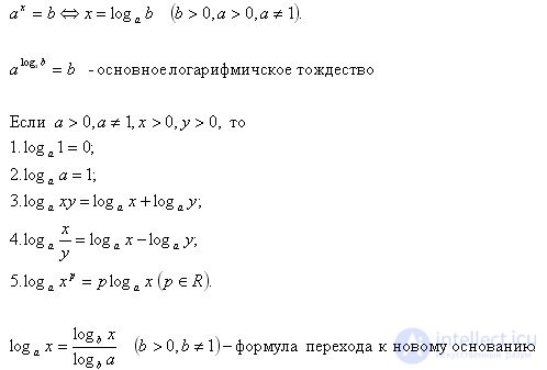
The basic logarithmic identity
The basic logarithmic identity follows from the definition of the logarithm[7]:
Corollary: if two real logarithms are equal, then the expressions under the logarithms are equal. Indeed, if , then , whence, by the basic identity: .
The intellectual source of, and stimulus for, the use of logarithms was the fact (already known to Archimedes[26]) that when powers are multiplied, their exponents add[27]:  . The 8th-century Indian mathematician Virasena, studying power relationships, published a table of integer exponents (that is, in effect, logarithms) for the bases 2, 3, 4[28].
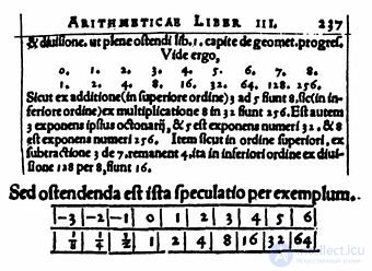
Logarithm table of M. Stifel, "Arithmetica integra", 1544
The decisive step was taken in medieval Europe. The need for complex calculations grew rapidly in the 16th century, and a considerable part of the difficulty came from multiplying and dividing multi-digit numbers and extracting roots. Toward the end of the century, several mathematicians, almost simultaneously, hit upon the idea of replacing laborious multiplication with simple addition, by using special tables to match a geometric progression with an arithmetic one, the geometric one being the original[26]. Division is then automatically replaced by the immeasurably simpler and more reliable subtraction, and raising to a power and extracting a root are simplified as well.
The first to publish this idea, in his book "Arithmetica integra" (1544), was Michael Stifel, who, however, made no serious effort to put his idea into practice[29][30]. Stifel's main merit is the transition from integer exponents to arbitrary rational ones[31] (the first steps in this direction were taken by Nicole Oresme in the 14th century and Nicolas Chuquet in the 15th century).
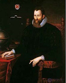
John Napier
In 1614 the Scottish amateur mathematician John Napier published, in Latin, a work titled "Description of the Wonderful Table of Logarithms" (Latin: Mirifici Logarithmorum Canonis Descriptio). It contained a brief description of logarithms and their properties, as well as 8-digit tables of logarithms of sines, cosines and tangents, with a step of 1'. The term logarithm, proposed by Napier, became established in science. Napier set out the theory of logarithms in another of his books, "Construction of the Wonderful Table of Logarithms" (Latin: Mirifici Logarithmorum Canonis Constructio), published posthumously in 1619 by his son Robert.
Judging by the documents, Napier had mastered the technique of logarithms as early as 1594[32]. The immediate purpose of developing it was to ease Napier's complex astrological calculations[33]; this is precisely why only logarithms of trigonometric functions were included in the tables.
The concept of a function did not yet exist, and Napier defined the logarithm kinematically, by juxtaposing uniform motion with logarithmically decelerating motion; for example, he defined the logarithm of a sine as follows[34]:
The logarithm of a given sine is the number which has increased arithmetically always at the same rate as that at which the total sine began to decrease geometrically.
In modern notation, Napier's kinematic model can be represented by a differential equation[35]:
 ,
,
where M is a scaling factor introduced so that the value would come out as an integer with the required number of digits (decimal fractions had not yet come into wide use). Napier took M = 10,000,000.
Strictly speaking, Napier tabulated not the function that is now called the logarithm. If we denote his function by  , then it is related to the natural logarithm as follows[35]:

Clearly,  , that is, the logarithm of the "total sine" (corresponding to 90°) is zero, which is exactly what Napier sought with his definition. He also wanted all logarithms to be positive; it is easy to verify that this condition holds for
  .
.  .
.
The basic property of Napier's logarithm: if quantities form a geometric progression, then their logarithms form an arithmetic progression. However, the rules for taking logarithms of Napier's function differed from those for the modern logarithm, for example:

As was soon discovered, because of an error in the algorithm, all values in Napier's table contained incorrect digits after the sixth place[36]. However, this did not prevent the new calculation method from gaining enormous popularity, and many European mathematicians took up compiling logarithm tables. In the astronomical handbook he published in 1620, Kepler inserted an enthusiastic dedication to Napier (not knowing that the inventor of logarithms had already died). In 1624 Kepler published his own version of logarithm tables (Latin: Chilias Logarithmorum ad totidem numeros rotundos)[37]. The use of logarithms allowed Kepler to complete relatively quickly his many years of work on the Rudolphine Tables, which cemented the success of heliocentric astronomy.
A few years after Napier's book, logarithm tables appeared that used an understanding of the logarithm closer to the modern one. The London professor Henry Briggs published 14-digit tables of decimal logarithms (1617), not for trigonometric functions but for arbitrary integers up to 1000 (seven years later Briggs extended the range to 20,000). In 1619 the London mathematics teacher John Speidell reissued Napier's logarithm tables, corrected and supplemented so that they effectively became tables of natural logarithms. Speidell's tables also included logarithms of the numbers themselves up to 1000 (and the logarithm of one, as in Briggs, was equal to zero), although Speidell retained the scaling to integers[38][39].
It soon became clear that the place of logarithms in mathematics is not limited to computational convenience. In 1629 the Belgian mathematician Grégoire de Saint-Vincent showed that the area under the hyperbola  varies according to a logarithmic law[40]. In 1668 the German mathematician Nicholas Mercator (Kauffman) discovered and published, in his book Logarithmotechnia, the expansion of the logarithm into an infinite series[41]. In the opinion of many historians, the appearance of logarithms had a strong influence on many mathematical concepts, including:
Until the end of the 19th century there was no generally accepted notation for the logarithm; the base a was written sometimes to the left of and above the symbol log, sometimes above it. In the end, mathematicians concluded that the most convenient place for the base is below the line, after the symbol log:  . Short notations for the most commonly used kinds of logarithm —
  for the decimal and natural logarithms — appeared much earlier, independently with several authors, and also became firmly established by the end of the 19th century[44].
An understanding of taking logarithms close to the modern one — as the operation inverse to exponentiation — first appeared with Wallis (1685) and Johann Bernoulli (1694), and was finally established by Euler[36]. In his book "Introduction to the Analysis of the Infinite" (1748), Euler gave the modern definitions of both the exponential and logarithmic functions, presented their expansions into power series, and especially noted the role of the natural logarithm[45]. Euler is also credited with extending the logarithmic function to the complex domain.
The first attempts to extend logarithms to complex numbers were made at the turn of the 17th and 18th centuries by Leibniz and Johann Bernoulli, but they failed to create a coherent theory, primarily because the very concept of the logarithm had not yet been clearly defined[46]. The discussion on this matter was held first between Leibniz and Bernoulli, and in the mid-18th century between d'Alembert and Euler. Bernoulli and d'Alembert held that one should define  , whereas Leibniz argued that the logarithm of a negative number is an imaginary number[46]. A complete theory of logarithms of negative and complex numbers was published by Euler in 1747–1751 and is essentially no different from the modern one[47]. Although the dispute continued (d'Alembert defended his point of view and argued it in detail in an article of his "Encyclopédie" and in other works), Euler's approach gained universal acceptance by the end of the 18th century.
In the 19th century, with the development of complex analysis, the study of the complex logarithm stimulated new discoveries. In 1811 Gauss developed a complete theory of the multivaluedness of the logarithmic function[48], defined as the integral of  . Riemann, building on the already known facts about this and similar functions, constructed the general theory of Riemann surfaces.
The development of the theory of conformal mappings showed that the Mercator projection in cartography, which arose even before the discovery of logarithms (1550), can be described as a complex logarithm[49].
Logarithmic functions are extremely widespread both in mathematics and in the natural sciences. Logarithms often appear where self-similarity is present, that is, where some object is repeatedly reproduced on a reduced or enlarged scale; see below such examples as recursive algorithms, fractals and mollusc shells. Here are several examples of the use of logarithms in various sciences.
Number theory
The distribution of prime numbers asymptotically obeys simple laws[50]:
 is approximately equal to
  .
. .
.Even more accurate estimates use the logarithmic integral.
A task that often arises is to roughly estimate a very large number — for example, a factorial or a Mersenne number with a large index. For this it would be convenient to write the number approximately in exponential format, that is, as a mantissa and a decimal exponent.
The task is easily solved using logarithms. Consider as an example the 44th Mersenne number  .
.

Therefore, the mantissa of the result is equal to {  Finally we obtain:

Mathematical analysis
See also: List of integrals of logarithmic functions
Logarithms often arise when finding integrals and solving differential equations. Examples:

Probability theory and statistics
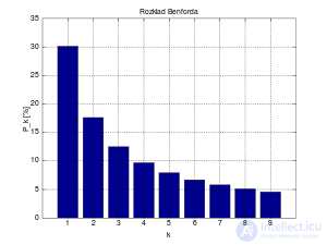
Benford's distribution. The horizontal axis shows the first significant digits, the vertical axis the probability of their occurrence.
In statistics and probability theory, the logarithm enters a number of practically important probability distributions. For example, the logarithmic distribution[51] is used in genetics and physics. The lognormal distribution often occurs in situations where the quantity under study is the product of several independent positive random variables[52].
Benford's law (the "first-digit law") describes the probability of a particular first significant digit appearing when real quantities are measured.
To estimate an unknown parameter, the maximum likelihood method and the associated log-likelihood function are widely used[53].
Fluctuations in a random walk are described by the Khinchin–Kolmogorov law.
Computer science and computational mathematics
In computer science: the unit of measurement of information (the bit). For example, to store a natural number  in a computer (in the usual binary format),
  bits are needed.
Information entropy is a measure of the amount of information.
Estimating the asymptotic complexity of recursive algorithms based on the "divide and conquer" principle[54] — such as quicksort, the fast Fourier transform, and so on.
Numerical values are usually stored in the memory of a computer or specialized processor in floating-point format. If, however, addition and subtraction are performed rarely on a group of data, while multiplication, division, exponentiation and root extraction are performed far more often, then it makes sense to consider storing such data in logarithmic format. In this case, instead of the number, the logarithm of its absolute value and its sign are stored, and thanks to the properties of the logarithm the speed of computation increases significantly[55]. The logarithmic storage format has been used in several systems, where it has proved effective[56][57].
Fractals and dimension
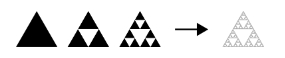
Sierpinski triangle (right)
Logarithms help express the Hausdorff dimension of a fractal[58]. For example, consider the Sierpinski triangle, which is obtained from an equilateral triangle by successively removing similar triangles, the linear size of each of which is halved at every stage (see the figure). The dimension of the result is determined by the formula:

Mechanics and physics
Boltzmann's principle in statistical thermodynamics defines entropy, one of the most important state functions of a thermodynamic system, characterizing its degree of disorder.
The Tsiolkovsky formula is used to calculate the velocity of a rocket.
Chemistry and physical chemistry
The Nernst equation relates the redox potential of a system to the activities of the substances involved in the electrochemical equation, as well as to the standard electrode potentials of the redox couples.
The logarithm is used in the definitions of such quantities as the autoprotolysis (self-ionization of a molecule) constant exponent and the hydrogen exponent (the acidity of a solution).
Music theory
To decide into how many parts the octave should be divided, one needs to find a rational approximation for 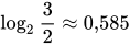 . If this number is expanded into a continued fraction, the third convergent (7/12) makes it possible to justify the classical division of the octave into 12 semitones[59].
Psychology and physiology
Human perception of many phenomena is well described by a logarithmic law.
The Weber–Fechner law is an empirical psychophysiological law stating that the intensity of a sensation is proportional to the logarithm of the intensity of the stimulus[60] — the loudness of a sound[61], the brightness of light.
Fitts's law: the farther away or the more precisely a movement of an organism is performed, the more correction is needed to carry it out, and the longer this correction takes[62].
The time needed to make a decision when there is a choice can be estimated by Hick's law[en][63].
Biology
A number of biological forms correspond well to the logarithmic spiral[64] — a curve whose tangent at every point makes the same angle with the radius vector at that point, that is, the increase of the radius per unit of circumference length is constant:
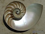
Nautilus shell
Arrangement of seeds on a sunflower

Romanesco cauliflower
Miscellaneous
The number of rounds in a single-elimination tournament equals the binary logarithm of the number of participants, rounded up to the nearest integer[65].
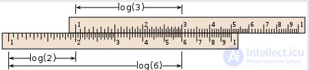
Logarithmic scale
The nonuniform scale of decimal logarithms is used in many areas of science. To facilitate calculations, it is marked on slide rules. Other examples:
The logarithmic scale is especially convenient when the levels of the measured quantity form a geometric progression, since their logarithms are then spaced at a constant step. For example, the 12 semitones of the classical octave form (approximately) such a progression[59] with common ratio  . Similarly, each level of the Richter scale corresponds to 10 times more energy than the previous level. Even in the absence of a geometric progression, a logarithmic scale can be useful for a compact representation of a wide range of values of the measured quantity.
The logarithmic scale is also widely used to estimate the exponent in power-law relationships and the coefficient in the exponent of an exponential. In this case a graph plotted on a logarithmic scale along one or both axes becomes a straight line, which is easier to study.
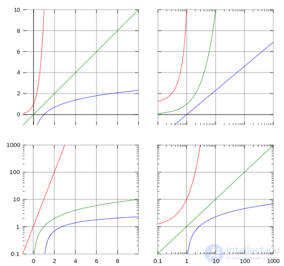
Graphs of three functions with different choices of scales on the coordinate axes:
Top row - 1) both linear; 2) logarithmic (x) and linear (y);
Bottom row - 1) linear (x) and logarithmic (y); 2) both logarithmic.

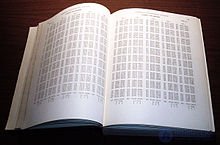
Logarithm tables
It follows from the properties of the logarithm that instead of laborious multiplication of multi-digit numbers, it suffices to look up (in the tables) and add their logarithms, and then, using the same tables (the "Antilogarithms" section), to perform exponentiation, that is, to find the value of the result from its logarithm. Division differs only in that the logarithms are subtracted.
The first tables of logarithms were published by John Napier (1614), and they contained only logarithms of trigonometric functions, and with errors at that. Independently of him, Jost Bürgi, a friend of Kepler, published his own tables (1620). In 1617 the Oxford professor of mathematics Henry Briggs published tables that already included decimal logarithms of the numbers themselves, from 1 to 1000, to 8 (later 14) places. But errors were found in Briggs's tables too. The first error-free edition, based on the tables of Georg Vega (1783), appeared only in 1857 in Berlin (Bremiker's tables)[76].
In Russia the first logarithm tables were published in 1703 with the participation of L. F. Magnitsky[77]. In the USSR several collections of logarithm tables were issued[78]:
The slide rule
In the 1620s Edmund Wingate and William Oughtred invented the first slide rule, which, until the appearance of pocket calculators, served as an indispensable calculating tool for engineers[79]. With this compact instrument one can quickly perform all algebraic operations, including those involving trigonometric functions[80]. The accuracy of the calculations is about 3 significant digits.
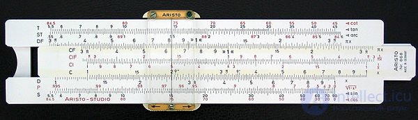
Slide rule. Multiplying 1.3 × 2 or dividing 2.6 / 2 (see scales C and D).
The logarithm, as a solution of the equation  , can be defined not only for real and complex numbers.
 are elements of a finite abelian multiplicative group, then the logarithm in this sense (if it exists) is called discrete. It is most often considered for the finite group of a residue ring modulo some number, where it is called the index modulo that number[82] and plays an important role in cryptography. In cyclic groups the logarithm exists if its base is a primitive root of the group.
Comments