
Lecture 23 min.
A quadratic equation is an algebraic equation of the general form

where  is the unknown,
  ,
,  ,
,  are coefficients, and
The expression 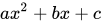 is called a quadratic trinomial .
A root is a value of the variable that turns the quadratic trinomial into zero, and the quadratic equation into a true numerical equality.
The elements of a quadratic equation have their own names :
is called the first or leading coefficient, is called the second or middle coefficient, or the coefficient of , is called the constant term.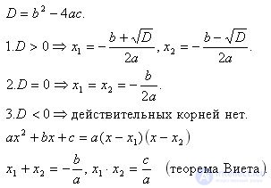
A quadratic equation whose leading coefficient equals one is called reduced (or monic) . Such an equation can be obtained by dividing the whole expression by the leading coefficient :

A quadratic equation all of whose coefficients are nonzero is called complete.
A quadratic equation in which at least one of the coefficients other than the leading one (either the second coefficient or the constant term) equals zero is called incomplete.
A quadratic equation is solvable in radicals, that is, its roots can be expressed in terms of the coefficients in a general form.
As early as the second millennium BC, the Babylonians knew how to solve quadratic equations . Solving them in Ancient Babylon was closely tied to practical problems, mainly such as measuring the area of plots of land and earthworks connected with military needs; this knowledge was also a result of the development of mathematics and astronomy in general. Methods were known for solving both complete and incomplete quadratic equations. Here are examples of quadratic equations solved in Ancient Babylon, written in modern algebraic notation:

The rules for solving quadratic equations are in many respects similar to modern ones, but the Babylonian texts do not record the reasoning by which these rules were obtained.
Problems solved with the help of quadratic equations appear in the astronomical treatise "Aryabhatiya," written by the Indian astronomer and mathematician Aryabhata in 499 AD. One of the first known derivations of the formula for the roots of a quadratic equation belongs to the Indian scholar Brahmagupta (around 598) ; Brahmagupta set out a universal rule for solving a quadratic equation reduced to the canonical form: 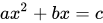 ; it was assumed that in it all coefficients except
  may be negative. The rule formulated by the scholar essentially coincides with the modern one.
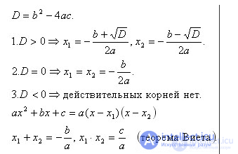
To find the roots of the quadratic equation  in the general case, one should use the algorithm below:
| Condition |  |
 |
 |
| Number of real roots | two roots | one root (in some contexts one also speaks of two equal or coinciding roots — it is also called a root of multiplicity 2) | we conclude that there are no roots over the real numbers. |
| Formula |
|
|
for the formula of complex roots, see the corresponding section below |
The formula can be obtained as follows:

We multiply each side by  and add
  :
:




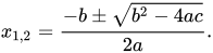
Note: it is clear that the formula for a root of multiplicity 2 is a special case of the general formula, obtained by substituting D=0 into it, and the conclusion that there are no real roots when D<0 should likewise be drawn by taking into account that in this case -D>0, and  .
.
The method presented is universal, but it is far from the only one.
For equations of the form  , that is, with an even , where

simpler expressions can be used to find the roots instead of formula (1) .
Note: the formulas given below can be obtained by substituting the expression b=2k into the standard formulas and carrying out some simple transformations.
|
Discriminant |
Roots |
|||
| non-reduced | reduced | D>0 | non-reduced | reduced |
| it is more convenient to compute the value of
a quarter of the discriminant:
All the necessary properties are preserved. |
 . . |
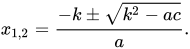 |
 |
|
| D=0 |  |
 |
Incomplete quadratic equations should be approached in a special way. Let us consider three possible situations.
|
b=0, c=0 |
b=0; c≠0 |
b≠0; c=0 |

(the transformation process is deliberately shown in detail; in practice one can go straight to the last equality) |

If |
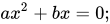
Such an equation always has two real roots |
There are special cases of quadratic equations in which the coefficients are related to one another in ways that allow them to be solved much more easily.
If in the quadratic equation the sum of the first coefficient and the constant term equals the second coefficient:  , then its roots are
  and the number opposite to the ratio of the constant term to the leading coefficient (
 ).
).
Way 1. First let us find out whether such an equation really has two roots (including two coinciding ones):
 .
.
Yes, it does, because for any real values of the coefficients  , and hence the discriminant is nonnegative. Thus, if
  , the equation has two roots, while if
  , it has only one root. Let us find these roots:
 .
.


In particular, if , there will be one root: 
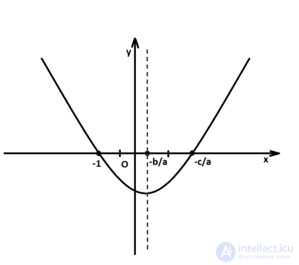
We use the geometric model of the roots of a quadratic equation: we will regard them as the points of intersection of the parabola  with the x-axis. Every parabola, regardless of the expression defining it, is a figure symmetric about the line
  . This means that the segment of any line perpendicular to it that is cut off by the parabola is bisected by the axis of symmetry. This holds, in particular, for the x-axis as well. Thus, for every parabola one of the following equalities holds:
 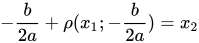 (if
(if  ) or
) or 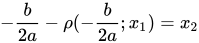 (if the inequality of the opposite sense holds). Using the identity
  , which expresses the geometric meaning of the absolute value, and also assuming that
  (this can be proved by substituting the equality into the quadratic trinomial:
  , so -1 is a root of such an equation), we arrive at the following equality:
  Taking into account that the difference is always positive when we add the absolute value and negative when we subtract it, which shows that these cases are equivalent, and, moreover, recalling the equality
  , we remove the absolute value:
  . In the second case, carrying out similar transformations, we arrive at the same result, Q.E.D.
Hence, before solving any quadratic equation, one should check whether this theorem can be applied to it: compare the sum of the leading coefficient and the constant term with the second coefficient.
If in a quadratic equation the sum of all its coefficients equals zero ( ), then the roots of such an equation are
  and the ratio of the constant term to the leading coefficient (
 ).
).
Way 1. First of all, note that the equality implies that 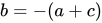 Let us determine the number of roots:

For any values of the coefficients the equation has at least one root: indeed, for any values of the coefficients , and hence the discriminant is nonnegative. Note that if , the equation has two roots, while if , it has only one. Let us find these roots:



which is what was to be proved.
In particular, if , the equation has only one root, which is the number .
Way 2. Using the definition of a root of a quadratic equation given above, we find by substitution that the number 1 is a root in the case under consideration:  is a true equality, so one is a root of equations of this kind. Next, by Vieta's theorem we find the second root: according to this theorem, the product of the roots of the equation equals the ratio of the constant term to the leading coefficient,
  , Q.E.D.
Hence, before solving an equation by standard methods, one should check whether this theorem applies to it: add up all the coefficients of the given equation and see whether this sum equals zero.
If a trinomial of the form  can somehow be represented as a product of linear factors
  , then the roots of the equation can be found: they will be
  and
and  ; indeed,
  , and by solving the indicated linear equations we obtain the above. Note that a quadratic trinomial cannot always be factored into linear factors with real coefficients: this is possible if the corresponding equation has real roots.
Let us consider some special cases.
If a quadratic trinomial has the form  , then by applying the named formula to it, we can factor it into linear factors and, therefore, find the roots:

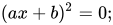

The same formula is also applied through the method called "completing the square" (of a sum or difference). For a reduced quadratic equation with the notation introduced earlier, this means the following:
 .
.
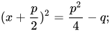
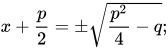
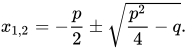
Note: as you may have noticed, this formula coincides with the one given in the section "Roots of the reduced quadratic equation," which, in turn, can be obtained from the general formula (1) by substituting the equality a=1. This is not just a coincidence: by the method described, with some additional reasoning, one can also derive the general formula and prove the properties of the discriminant.
Vieta's theorem (see the section of the same name below) and its converse allow reduced quadratic equations to be solved mentally, without resorting to computation by formula (1).
According to the converse theorem, any pair of numbers (or single number)  , being a solution of the system of equations
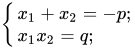
are the roots of the equation  .
.
The direct theorem helps in finding, mentally, numbers that satisfy these equations. With its help one can determine the signs of the roots without knowing the roots themselves. To do so, follow this rule:
1) if the constant term is negative, the roots have different signs, and the root with the larger absolute value has the sign opposite to that of the second coefficient of the equation;
2) if the constant term is positive, both roots have the same sign, and it is the sign opposite to that of the second coefficient.
The so-called "transfer" method makes it possible to reduce the solution of non-reduced equations, which cannot be converted to reduced form with integer coefficients by dividing by the leading coefficient, to the solution of reduced equations with integer coefficients. It consists of the following:
1) multiply both sides by the expression:


2) introduce a new variable  :
:

Next, the equation is solved mentally in the way described above, then one returns to the original variable and finds the roots of the equations  and
and  .
.
Suppose we want to solve the equation  using the converse of Vieta's theorem. If we try to divide both sides by 8, we obtain a reduced equation with fractional coefficients, so it will be hard to apply the theorem to it. However, by using the transfer method, we can obtain a reduced equation with integer coefficients:

 .
.
Making the change of variable y=8x, we arrive at the equation:
 .
.
Clearly, its roots are the numbers -4 and 2. We now perform the reverse substitution:


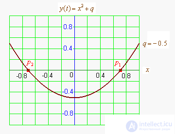
The graph of a quadratic function is a parabola. The solutions (roots) of a quadratic equation are the abscissas of the points where the parabola crosses the x-axis. If the parabola described by the quadratic function does not intersect the x-axis, the equation has no real roots. If the parabola meets the x-axis at one point (the vertex of the parabola), the equation has one real root (one also says that the equation has two coinciding roots). If the parabola crosses the x-axis at two points, the equation has two real roots (see the image on the right.)
If the coefficient is positive, the branches of the parabola point upward, and vice versa. If the coefficient is positive (for positive ; for negative, the opposite), then the vertex of the parabola lies in the left half-plane, and vice versa.
Besides the universal method described above, there is the so-called graphical method. In general, this method of solving a rational equation of the form  consists of the following: the graphs of the functions
  and
and  are plotted in one coordinate system, and the abscissas of the common points of these graphs are found; the numbers found are the roots of the equation.
There are only five main ways to solve quadratic equations graphically.
To solve the quadratic equation by this method, the graph of the function is plotted and the abscissas of the points where this graph meets the -axis are found.
To solve the same equation by this method, it is transformed to the form  and the graphs of the quadratic function
  and the linear function
  are plotted in one coordinate system, and then the abscissas of their intersection points are found.
Solving by this method involves transforming the original equation to the form  using the method of completing the square (of a sum or difference), and then to
  . After that, the graph of the function
 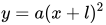 is plotted (it is the graph of the function shifted by
  scale units to the right or to the left, depending on the sign), together with the line
  , parallel to the x-axis. The roots of the equation are the abscissas of the points where the parabola and the line intersect.
The quadratic equation is transformed to the form  , the graph of the function
  is plotted (it is the graph of the function shifted by scale units upward if this coefficient is positive, or downward if it is negative), along with
  , and the abscissas of their common points are found.
The quadratic equation is transformed to a special form:
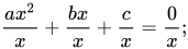
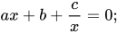
then
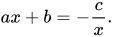 .
.
After performing the transformations, the graphs of the linear function  and the inverse proportionality
 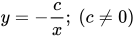 are plotted, and the abscissas of the intersection points of these graphs are found. This method has a limit of applicability: if
  , the method is not used.
The graphical methods described above have significant drawbacks: they are quite laborious, and the accuracy of constructing the curves, parabolas and hyperbolas, is low. These problems do not affect the method proposed below, which relies on relatively more accurate constructions with a compass and straightedge.
To carry out such a solution, the following sequence of steps must be performed.
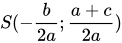 , passing through the point C(0;1) on the y-axis.
 .
.A quadratic equation with real coefficients  has exactly two complex roots, as the fundamental theorem of algebra states. Depending on the value of the discriminant
 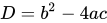 , either one or both roots may have no imaginary part and be real:
there are two real roots, and they are computed by the formula
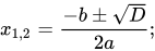
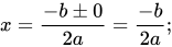
there is one root (which can also be described as two equal or coinciding roots), of multiplicity 2:
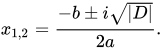
there are no real roots, but there are two complex roots, expressed by the same formula as for a positive discriminant. It can also be rewritten by expressing the square root of a negative number as the product of a root and the imaginary unit:
In the complex case, a quadratic equation is solved by the same formula (1) and its variants given above, but only two cases can be distinguished: a zero discriminant (one double root) and a nonzero discriminant (two simple roots).
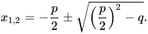
A quadratic equation of the form  in which the leading coefficient equals one is called reduced (or monic). In this case the formula for the roots (1) simplifies to
Mnemonic rules:
Write a "minus" first,
Next to it p halved,
"Plus-minus" the radical sign,
Familiar to us since childhood.
And under the root, my friend,
It all comes down to a trifle:
p halved and squared
Minus the lovely q.
p, taken with the opposite sign,
We will divide by two,
And from the root, carefully,
We will separate it with a "minus-plus" sign.
And under the root, quite conveniently,
Half of p squared
Minus q — and there are the solutions,
That is, the roots of the equation.
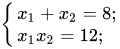
The sum of the roots of the reduced quadratic equation is equal to the coefficient  taken with a minus sign, and the product of the roots is equal to the constant term

In the general case, that is, for a non-reduced quadratic equation :

Using this theorem, some quadratic equations can be solved mentally.


If both roots of a quadratic trinomial are known, it can be factored using the formula
 (2)
(2)
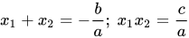
To prove this statement, we use Vieta's theorem. According to this theorem, the roots  and
and  of the quadratic equation satisfy the following relations with its coefficients:
  . Let us substitute these relations into the quadratic trinomial:

 .
.
In the case of a zero discriminant, this relation becomes one of the forms of the square of a sum or difference formula.
Two important corollaries follow from formula (2):
If a quadratic trinomial factors into linear factors with real coefficients, then it has real roots.
Let  . Then, rewriting this factorization, we obtain:
 .
.
Comparing the resulting expression with formula (2), we find that the roots of such a trinomial are and  . Since the coefficients are real, the numbers opposite to their ratios are also elements of the set .
If a quadratic trinomial has no real roots, then it does not factor into linear factors with real coefficients.
Indeed, if we assume the contrary (that such a trinomial factors into linear factors), then, by Corollary 1, it has roots in the set , which contradicts the hypothesis; therefore our assumption is false, and such a trinomial does not factor into linear factors.
An equation of the form  is an equation reducible to a quadratic one.
In the general case it is solved by the substitution  followed by solving the quadratic equation
  .
.
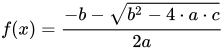
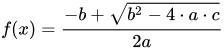
It is also possible to solve it without a substitution, by solving a system (union) of two equations:
 and
and
If  , then the equation takes the form:

Such an equation is called biquadratic .
By means of the substitution

the following equation is reduced to a quadratic equation

known as a reciprocal (or generalized symmetric) equation .
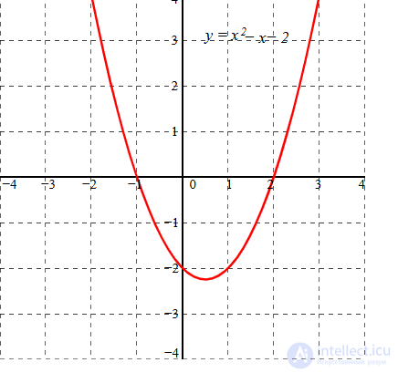
For the quadratic function:
f (x) = x2 − x − 2 = (x + 1)(x − 2) of a real variable x, the x-coordinates of the points where the graph crosses the x-axis, x = −1 and x = 2, are the solutions of the quadratic equation: x2 − x − 2 = 0.
A second-order linear homogeneous differential equation with constant coefficients

is reduced by the substitution  to the characteristic quadratic equation:

If the solutions of this equation  and
and  are not equal to each other, then the general solution has the form:
 , where
  and
and  are arbitrary constants.
For complex roots  the general solution can be rewritten using Euler's formula:

If the solutions of the characteristic equation coincide,  , the general solution is written in the form:

Equations of this type often occur in a wide variety of problems in mathematics and physics, for example, in the theory of oscillations or the theory of alternating current circuits.
Solving quadratic equations has many practical applications in various fields. Here are some of the main ones:
These examples show that quadratic equations are essential for analyzing and solving problems in science, engineering, business and other practical fields where a quadratic dependence is present.
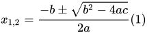
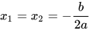
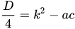


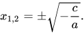
 , then the equation has two real roots, and if
  , then the equation has no real roots.
 or
or 

Comments