
Lecture
Let us consider the features of the continuous-deterministic approach, using as an
example the use of differential equations as mathematical models. Differential equations are equations in which the unknowns are functions of one or several variables, and the equation contains not only the functions themselves but also their derivatives of various orders. If the unknowns are functions of many variables, the equations are called partial differential equations; otherwise,
when a function of only one independent variable is considered, the equations
are called ordinary differential equations.
Usually, in such mathematical models time t serves as the independent variable on which the unknown sought functions depend. Then the mathematical relationship for deterministic systems (6) will, in general
form, be

where
y'
= dy/dt, y
= (y1, y2, ..., yn)
and
f
= (f1, f2, ..., fn) – n-dimensional vectors;
f(y,t) – a continuous vector-function defined on
an (n+1)-dimensional set.
Since mathematical schemes of this kind reflect the dynamics of the system under study, i.e. its behaviour over time, they are called D-schemes
(from the English word dynamic).
In the simplest case, an ordinary differential equation has the form
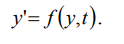 (8)
(8)
Of greatest importance for systems engineering is the application of D-schemes as a mathematical apparatus in automatic control theory. To illustrate the features of constructing and applying D-schemes, let us consider the simplest
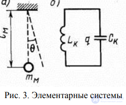
example of formalising the operating process of two elementary systems
of different physical nature: a mechanical one
(pendulum oscillations, Fig. 3 (a)) and an electrical one
(an oscillating circuit, Fig. 3 (b)).
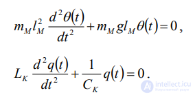
The process of small pendulum oscillations and
the process in the electrical oscillating circuit
are described by ordinary differential equations (see Fig. 3)
.
Introducing the corresponding notation in the above equations, we obtain a second-order ordinary differential equation describing the behaviour of this closed system
 , (9)
, (9)
where
h0,
h1,
h2 — parameters of the system;
z(t) — the state of the system at time t.
Thus, the behaviour of these two objects can be investigated
on the basis of the common mathematical model (9). It should also be noted that the behaviour of one of the systems can be analysed using
the other. For example, the behaviour of the pendulum can be studied using the electrical oscillating circuit.
If the system under study S, i.e. the pendulum or the circuit, interacts with
the external environment E, an input action appears
x(t)
(an external force for
the pendulum and a source of energy for the circuit), and the continuous-deterministic
model of such a system will have the form

From the point of view of the general scheme of the mathematical model,
x(t)
is
an input action, and the state of the system S can in this case be consid Fig. 3. Elementary systems
ered as an output characteristic, i.e. it is assumed that the output variable
coincides with the state of the system at the given moment in time
y = z.
In solving systems-engineering problems, the problems of
controlling large systems are of great importance. Attention should be paid to automatic control systems — a special case of dynamic systems described by D-schemes and singled out as a separate class of models because of their practical specifics.
In describing automatic control processes, it is customary to adhere
to a representation of the real object as two systems: a controlling one and
a controlled one (the control object). The structure of a general multidimensional automatic control system is shown in Fig. 4, where the following are denoted:
endogenous variables:
x(t) — the vector of input (reference) actions;
υ(t) — the vector of disturbing actions;
h'(t) — the vector of error signals;
h''(t) — the vector of control actions;
exogenous variables:
z(t) — the vector of states of the system S;
y(t) — the vector of output variables, usually
y(t) = z(t).
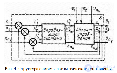
Fig. 4. Structure of an automatic control system
A modern control system is a set of software and hardware tools that ensure the control object achieves a cer
tain goal. How precisely the control object achieves the assigned goal,
can be judged, for a one-dimensional system, from the state coordinate
y(t). The difference
between the assigned
y des(t)
and the actual
y(t)
laws of variation of the controlled quantity is the control error
h'(t)
= y des(t) - y(t). If the prescribed
law of variation of the controlled quantity corresponds to the law of variation of the input (reference) action, i.e.
x(t) = y des(t)
, then
h'(t) = x(t) - y(t).
Systems for which the control errors
h'(t) = 0
at every moment in time are called ideal. In practice, the realisation of ideal systems is impossible. Thus, the error
h'(t) — a necessary substrate of automatic control based on the principle of negative feedback, since
bringing the output variable
y(t)
into correspondence with its assigned
value requires information about the deviation between them. The task of the automatic control system is to change the variable
y(t)
according to the assigned law with a certain accuracy (within a permissible error).
When designing and operating automatic control systems, it is necessary to choose such parameters of the system S as would ensure the required control accuracy, as well as the stability of the system in the transient process.
If the system is stable, then of practical interest are the behaviour of the system over time, the maximum deviation of the controlled variable
y(t)
in the transient process, the duration of the transient process, and so on. Conclusions about the properties of automatic control systems of various classes can be drawn from
the form of the differential equations that approximately describe the processes in
the systems. The order of the differential equation and the values of its coefficients are fully determined by the static and dynamic parameters of the system S.

Comments