
Lecture
We shall consider the features of the continuous-stochastic approach using, as an
example, the application of queueing systems as standard mathematical schemes (queueing systems), which we shall call Q-schemes. Queueing systems form a class of mathematical schemes developed in queueing theory and in various
applications for the formalisation of the operating processes of systems that
are, in essence, service processes.
As a service process one may represent various
operating processes, differing in their physical nature, of economic,
production, technical and other systems, for example, flows of supplies
of production to some enterprise, flows of parts and components on an assembly-line conveyor, requests for information processing by a computer from
remote terminals, and so on. A characteristic feature of the operation of such objects is the random appearance of requests (demands) for service and the completion of service at random instants of time, i.e. the stochastic
nature of their operating process. Let us dwell on the basic concepts of
queueing needed for the use of Q-schemes, both in
analytical and in simulation modelling.
In any elementary act of service two main components can be distinguished: the request's waiting for service and the service itself. This can be depicted as some i-th service device
Pi (Fig. 5), consisting
of a queue of requests Hi
, in which
there may simultaneously be present
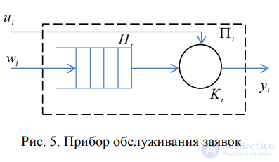 Fig. 5. Service device for requests
Hi
LiH
l ≥ 0,
of requests, where
LiH
— the capacity of the i-th queue, and of the service channel for requests (or simply the channel) Ki
. Onto each element of the service device Pi there arrive flows of events: into the queue Hi
— the flow of requests wi; onto the channel Ki — the service flow.
A flow of events is the name given to a sequence of events occurring one after another at some random instants of time. A distinction is made between flows of homogeneous and inhomogeneous events. A flow of events is called homogeneous if it is characterised only by the instants of occurrence of these events
(the calling instants) and is given by the sequence
t
1 ≤ 0 ≤ t
2 ≤ t
3
... ≤ t
n ≤ ...
, where
n
t — the instant of occurrence of the n-th event — a nonnegative real number. A homogeneous flow of events can also be
given in the form of a sequence of time intervals between the n-th and the (n—1)-th
events
τn, which is uniquely related to the sequence of calling instants
t
n
, where
τn
= t
n − t
n-1
, n ≥ 1, t
0 = 0
, i.e.
τ1
= t1 .
A flow of inhomogeneous events is the name given to the sequence
t
n
, f
n ,
where
n
t – the calling instants;
n
f — the set of the event's attributes. For example,
as applied to the service process, for an inhomogeneous flow of requests one may specify membership of one or another source of requests, the presence of a
priority, and the possibility of service by one or another type of channel, and so on.
Usually, in applications, when modelling various systems, for an elementary service channel Ki one can assume that the flow of requests
wi ∈ W, i.e. the time intervals between the instants of appearance of requests (the calling instants) at the input of Ki form a subset of uncontrollable variables, while the service flow
ui ∈ U, i.e. the time intervals between the start and
the completion of service on a request forms a subset of controlled variables.
Requests serviced by the channel Ki, and requests that left the device Pi
unserviced for various reasons (for example, because of an overflow of the queue
of Pi), form the output flow
yi ∈ Y, i.e. the time intervals between the instants of departure of requests form a subset of output variables.
The operating process of the service device Pi can be represented as the process of change of the states of its elements over time
z t i
. A transition
to a new state for Pi means a change in the number of requests present in it
(in the channel Ki and in the queue Hi
. Thus, the state vector for
Pi has the form
K
i
H
i
zi = z ,z , where
H
i
z — the state of the queue Hi (
0
H
i
z – the queue is empty,
1
H
i
z – there is one request in the queue,
H
i
H
zi
= L – the queue is completely full);
H
Li — the capacity of the queue Hi
, measured by the number of requests that can fit into it;
K
i
z — the state of the channel Ki (
0
K
i
z — the channel is free,
1
K
i
z — the channel is busy, and so on).
In the practice of system modelling, for systems with more complex structural links and behaviour algorithms, it is not individual service devices that are used for formalisation but Q-schemes, formed by a composition of many elementary service devices Pi (queueing networks). If
the channels Ki of various service devices are connected in parallel, then this is
multichannel service (a multichannel Q-scheme), and if the devices Pi and their parallel compositions are connected in series, then this is multiphase service (a multiphase Q-scheme). Thus, to define a Q-scheme it is necessary to use a coupling operator R, reflecting
the interrelation of the structural elements (channels and queues) with one another.
Connections between the elements of a Q-scheme are depicted as arrows (flow lines
reflecting the direction of movement of requests). A distinction is made between open and
closed Q-schemes. In an open Q-scheme the output flow of serviced requests cannot re-enter any element, i.e. there is no feedback, whereas in closed Q-schemes there are feedback connections along which requests
move in the direction opposite to the input-output movement.
The inhomogeneity of requests, reflecting the process in one or another real
system, is taken into account by introducing priority classes. Depending
on the dynamics of priorities, a distinction is made in Q-schemes between static and dynamic
priorities. Static priorities are assigned in advance and do not depend on the states of the Q-scheme, i.e. they are fixed within the limits of solving a particular modelling problem. Dynamic priorities arise during modelling depending on the situations that occur. Based on the rules for selecting requests from the queue for service by the channel Ki
, one can distinguish relative and absolute priorities. A relative priority means that
a request with a higher priority, arriving in the queue Hi, waits
for the completion of service of the preceding request by the channel Ki and only after
that occupies the channel. An absolute priority means that a request with a higher priority, arriving in the queue Hi
, interrupts service
by the channel Ki
, of a request with a lower priority, and itself occupies the channel (in
this case the request displaced from Ki may either leave the system or may be
written again to some place in Hi
.
When considering the algorithms of operation of the service devices Pi (channels Ki and queues Hi) it is also necessary to specify a set of rules by
which requests leave Hi
, and Ki. In addition, for requests it is also necessary
to specify
the rules by which they remain in the channel Ki or are not admitted to service by the channel Ki, i.e. the rules of channel blocking. Here a distinction is made between blockings of Ki by output and by input. Such blockings reflect the presence of control links in the Q-scheme, regulating the flow of requests depending on the states of the Q-scheme. The whole set of possible algorithms of request behaviour in the Q-scheme
can be represented in the form of some operator of algorithms of request behaviour
A.
Thus, a Q-scheme, describing the operating process of a queueing system of any complexity, is uniquely given in the form
Q = W,U,H,Z,R, A .
In the practice of modelling objects one often has to solve problems,
connected with the formalised description and analysis of cause-and-effect
relations in complex systems, where several processes proceed simultaneously in parallel.
The most widespread formalism at present, describing the structure and interaction of parallel systems and processes, is Petri nets (Petri Nets).
The theory of Petri nets is developing in several directions: the development
of mathematical foundations, the structural theory of nets, various applications (parallel programming, discrete dynamic systems, and so on).
Formally a Petri net (an N-scheme) is given by a quadruple of the form
N = B,D,I,O ,
where B — a finite set of symbols called places, B≠Ø; D — a finite set of symbols called transitions, D≠Ø, B∩D≠Ø; I—
the input function (the direct incidence function), I: B x D→{0, 1}; O — the output function (the inverse incidence function), O: D x B→ {0, 1}. Thus
, the input function maps a transition
dj
to the set of its input places
I(dj), while the output function O maps a transition
dj
to the set of its output places
O(dj)
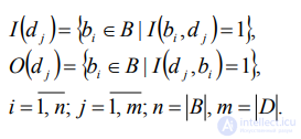
. For each transition
dj D
one can define
the set of input places of the transition
I(dj)
and
the set of output places of the transition
O(dj) as
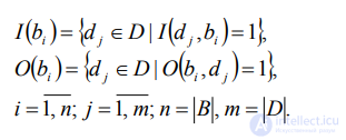
Similarly, for each transition
bi B
definitions are introduced of the set of input transitions
of a place I(bi)
and of the set of output transitions
of a place
Graphically an N-scheme is depicted as a bipartite directed multigraph, representing a collection of the places and transitions of the N-scheme (Fig. 6). As is evident from this figure,
the graph of an N-scheme has two types of nodes: places and
transitions, depicted as 0 and 1 respectively.
Directed arcs connect places and
transitions, with each arc directed from
an element of one set (a place or a transition) to an element of the other set (a transition or a place). The graph of an N-scheme is a multigraph, since it
admits the existence of multiple arcs from one vertex to another.
The representation of an N-scheme given above can be used only
to reflect the statics of the modelled system (the interrelations of events and conditions),
but does not allow the dynamics of the operation of the modelled
system to be reflected in the model. To represent the dynamic properties of the object, a marking function is introduced:
M: B→{0, 1, 2, ...}. A marking M is the assignment
of certain abstract objects, called tokens (markers), to the places of the N-scheme, and the number of tokens corresponding to each place may change. In the graphical representation of an N-scheme, a marking is depicted by placing
the corresponding number of dots inside the place-vertices (when the number of dots is large, numerals are used instead).
A marked N-scheme can be described in the form
N = B,D,I,O,M .
The operation of an N-scheme is reflected by way of a transition from one marking to
another. The initial marking is denoted as M0: B→ {0, 1, 2, ...}. A change of markings occurs as a result of the firing of one of the transitions
dj D
of the net.
A necessary condition for the firing of a transition
dj
is that
for every bi I(dj), M(bi)
1,
where
M(bi) — the marking of the place
bi. A transition
dj, for which the stated condition holds, is defined as being in a state of readiness to fire, or as an enabled transition.
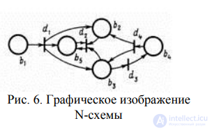
Fig. 6. Graphical depiction
of an N-scheme
The firing of a transition
dj
changes the marking of the net
M(b1), M(b2), ..., M(bn)
,
to the marking M'(b) according to the following rule:
M'(bi) = M(bi) minus I(dj, bi) plus O(dj, bi),
i.e. the transition
dj
removes one token from each of its input places and
adds one token to each of the output places. To depict
a change of marking from M to M' the notation is used
dj
M -> M'.
Thus, an N-scheme operates by way of the firing of transitions, under
the control of the number of tokens and their distribution in the net. A transition is fired
by removing tokens from its input places and forming new tokens, placed in the output places. A transition can be fired only when
it is enabled. A transition is called enabled if each of its input
places has a number of tokens at least equal to the number of arcs from the place to the transition.
An important feature of models of the operating process of systems
using standard N-schemes is the simplicity of constructing hierarchical
structures of the model. On the one hand, every N-scheme can be regarded
as a macro-transition or macro-place of a model of a higher level. On the other
hand, a transition, or a place of an N-scheme, can be elaborated in the form of a separate subnet for a more detailed study of the processes in the modelled system. From this follows the possibility of effectively using N-schemes for modelling parallel and competing processes in various systems.
The most well-known general approach to the formal description of the operating processes of systems is the approach proposed by
N. P. Buslenko. This approach makes it possible to describe the behaviour of continuous and discrete,
deterministic and stochastic systems, i.e. compared with those considered, it is generalised (universal) and is based on the concept of
of an aggregative system (from aggregate system), representing a formal scheme of a general form, which we shall call an A-scheme
An analysis of the existing means of modelling systems and of the problems solved with the help of the method of computer modelling inevitably leads to the conclusion
that a comprehensive solution of the problems arising in the process of creating and computer-implementing a model is possible only if the modelling systems have at their basis a single formal mathematical scheme, i.e.
an A-scheme. Such a scheme must simultaneously perform several functions:
to be an adequate mathematical description of the object being modelled, i.e. of the system S;
to serve as the basis for constructing algorithms and programs in
the computer implementation of the model M;
to allow, in a simplified variant, analytical
studies to be carried out.
In an aggregative description a complex object (system) is broken down into
a finite number of parts (subsystems), while preserving the links ensuring
their interaction. If some of the resulting subsystems turn out in
their turn to be still fairly complex, the process of their decomposition continues until subsystems are formed which, under the conditions of the modelling problem in question, can be regarded as convenient for a mathematical
description. As a result of such decomposition a complex system is represented in
the form of a multilevel structure of interconnected elements, united into subsystems of various levels.
As an element of an A-scheme there acts an aggregate, and the connection between aggregates (within the system S and with the external environment E) is realised by means of the coupling operator R. Obviously, an aggregate can itself be regarded as an A-scheme, i.e. it can be broken down into elements (aggregates) of the next level.
Any aggregate is characterised by the following sets: of instants
of time T, of input X and output Y signals, of states Z at each
instant
of time t. The state
of the aggregate at the
instant of time t belongs
to T is denoted as
z(t) belongs to Z, while
the input and output signals
— as x(t) belongs to
X and y(t) belongs to
Y respectively. Let us assume
that the transition of the
aggregate from the state z(t1)
to the state z(t2) greater
than z(t1) takes place over
a small interval of time,
i.e. a jump z occurs.
Transitions of the aggregate from
state to state are
determined by the aggregate's
own (internal) parameters h(t)
belongs to H and
by the input signals
x(t) belongs to X.
At the initial instant
of time t0 the
states z have values
equal to z0, i.e.
z0 = z(t0), given
by the distribution law
of the process z(t)
at the instant of
time t0, namely L[z(t0)].
Let us suppose that
the operating process of
the aggregate, in the
case of the action
of the input signal
xn, is described by
the random operator V.
Then, at the instant
of arrival at the
aggregate tn belongs to
T of the input
signal xn, one can
determine the state z(tn
+ 0) = V[t,
z(tn), xn]. If the
interval of time (tn,
tn+1] does not contain
a single instant of
arrival of signals, then
for t belongs to
(tn, tn+1] the state
of the aggregate is
determined by the random
operator U in accordance
with the relation z(t)
= U[t, tn, z(tn
+ 0)]. The set
of random operators V
and U is regarded
as the operator of
transitions of the aggregate
into new states. Here
the operating process of
the aggregate consists of
jumps of state z
at the instants of
arrival of input signals
x (the operator V)
and of changes of
state between these instants
tn and tn+1 (the
operator U). No restrictions
are imposed on the
operator U, so jumps
of state δz are
permissible at instants of
time that are not
instants of arrival of
input signals x. Subsequently
the instants of jumps
δz will be called
special instants of time
t*, and the states
z(t*) — special states of the A-scheme. To describe
jumps of state z at special instants of time,
we shall use the random operator W, which is
a particular case of the operator U, i.e. z(t*
+ 0) = W[t*, z(t*)]. In the set of
states Z one distinguishes such a subset Y that
is a subset of Z that, if z(t) reaches
Y that is a subset of Z, then this
state is the instant of issuing an output signal,
determined by the output operator y = G[t, z(t)].
Thus, by an aggregate we shall mean any object
defined by an ordered set of the sets considered,
T, X, Y, Z, ZY, H, and of the
random operators V, U, W, G. A sequence of
input signals, arranged in the order of their arrival
at the A-scheme, we shall call an input message,
or an x-message. A sequence of output signals, ordered
with respect to the time of issue, we shall
call an output message, or a y-message. There exists
a class of large systems which, owing to
their complexity, cannot be formalised in the form
of mathematical schemes of single aggregates, therefore they
are formalised by a certain construction of separate
aggregates An, n = 1, NA, which we
shall call an aggregative system or an A-scheme.
To describe a given real system S in
the form of an A-scheme it is necessary
to have a description both of the individual
aggregates An and of the connections between them.

Comments