
Lecture 52 min.
The assumption that molecules are uniformly distributed in space and that their velocities are uniformly distributed over all directions is called the molecular chaos assumption. Strange as it may seem, it is precisely because the motion of molecules is absolutely chaotic that one can establish definite regularities governing the state of the system. In addition, in practice one often has to deal with a gas placed in a uniform external force field, the most important example of which is the gravitational field.
Suppose there is a closed vessel of small volume (so that the action of external force fields can be neglected) filled with gas. Assume that the gas has reached a state of equilibrium.
|
The equilibrium state of a system is a state in which all parameters of the system have definite values that remain constant for arbitrarily long times under unchanging external conditions. |
The external conditions must be such that there is no transport of matter, energy, momentum, etc. in the system.
Video 3.1. Fluctuations in the number of molecules in half of the vessel are quite noticeable if the number of molecules is small.
Experiment shows that at equilibrium, in the absence of external force fields:
|
|
|
(3.1) |
Video 3.2. The chaotic motion of molecules leads to their uniform distribution throughout the volume of the vessel. When the number of molecules is large, fluctuations of their number in half of the vessel are insignificant.
This means that the number of molecules moving in any direction must be the same. If this were not so and there were a direction of preferential motion of the molecules, a flow of gas would arise in that direction, which contradicts the assumption that equilibrium exists.
Within any solid angles, however oriented but equal in magnitude, lie the directions of motion of, on average, the same number of molecules (Fig. 3.1).
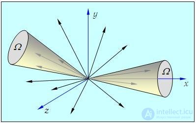
Fig. 3.1. Distribution of molecules by direction of motion
Collisions of molecules do not change this situation. For simplicity we will consider an ideal gas. From the standpoint of kinetic theory, an ideal gas is the simplest molecular-kinetic model of a gas.
As noted earlier, the ideal gas model assumes the following two properties:
Real gases are close to an ideal gas at low densities. As the density decreases, the average distances between molecules become much greater than the linear dimensions of the molecules, and the interaction force between them decreases practically to zero.
Distribution function. What is a distribution? Let us begin with a simple example that allows us to formulate the necessary definitions. Suppose that in some group of 100 people, 10 have a height from 160 to 165 cm, 25 from 165 to 170, 35 from 170 to 175, 15 from 175 to 180, 10 from 180 to 185, and the remaining 5 from 185 to 190. It is convenient to represent this enumeration as a simple, commonly used diagram, drawing vertical rectangles with height proportional to the number of people of a given height (Fig. 3.2). Such a diagram is called a histogram. If we construct it not for a hundred people but for the adult population of an entire country, we can introduce much finer subdivisions of height. For example, we could determine height to an accuracy not of 5 cm but of 0.5 cm (for human height, greater accuracy hardly makes sense).
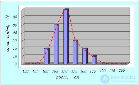
Fig. 3.2. A histogram showing the distribution of people by height, and the approximate form of the corresponding distribution function (dashed curve)
Video 3.3. Random collisions are not limited to those of gas molecules with one another: "generating" a Gaussian distribution with millet grains.
Let us assume, however, that the quantity under study can be specified arbitrarily accurately, so that for a very large group it is legitimate to pass from the histogram to a smooth distribution function, whose graph passes through the midpoints of the upper sides of the vertical rectangles of the histogram (the dashed curve in Fig. 3.2). It is precisely a curve of this kind that we must construct for the distribution of gas molecules over velocities.
Random events. The branch of mathematics that studies random phenomena is called probability theory. Its basis is the concept of a random event as one of the possible outcomes of some trial — a process that can in principle be reproduced an unlimited number of times. At an intuitive level this concept is clear, and we will not go into its formal definition adopted in modern mathematics. Rolling a 6 (or any other number) when throwing a die, or the appearance of red or black in roulette, are examples of random events.
Often, however, we deal with non-reproducible events to which probability theory is nevertheless applicable. This concerns the quantitative characteristics of mass phenomena. Say, a factory manufactures a transistor. It may be defective or working, but unlike throwing a die, it is no longer possible to repeat the process and make the very same transistor a second, third, ..., millionth time. To the same class of phenomena belong the occurrence of a given number of calls at a telephone exchange, the age of a person occupying a particular seat in a stadium of a hundred thousand, and so on.
Can random events or mass phenomena be described by mathematical formulas? Can regularities be found in the world of chance? Such attempts have been made since antiquity because of practical needs. Already in ancient states, forecasts were made of population growth and of the amount of harvest and taxes collected. The development of insurance in the Middle Ages required an assessment of the danger of shipwreck. In the 17th century the first life insurance society was founded in Italy, and its founder needed to know the risk of a client's death depending on his age and occupation. The final impetus for the emergence of probability theory as an independent mathematical discipline was the spread of gambling.
Probability of a random event. To each random event one can assign a number called the probability of the event. The probability of a random event is determined by the relative frequency of its occurrence among other random events. The more often an event occurs, the greater its probability.
Suppose some trial is performed whose outcome is some set of random events A, B, C, .... Say, a die is thrown, assumed to be geometrically regular, so that all its faces are equivalent. There are six possible events in all — the numbers 1, 2, ..., 6 coming up. Suppose n trials have been performed, and event A occurred kn(A) times. The quantity
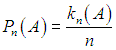
is the relative frequency of event A in the given series of trials. Generally speaking, the value of Pn(A) fluctuates from one series of trials to another. If, as the number n of trials in the series increases, the number Pn(A) tends to a definite limit
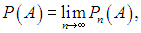
then this limit P(A) is called the probability of event A. If the die is thrown sufficiently many times in our example, the frequency of each of the numbers will be the same. We say that the probability of any of them coming up is 1/6.
It follows from the classical definition of probability that it always lies between zero and one:

|
The probability of an impossible event is zero; the probability of a certain event is one. |
The converse statements are, generally speaking, false. For example, one should not think that an event whose probability is zero can never occur. The events that occur when a die is thrown are discrete: a one or a two may come up, but not two and a half. But what should we do if the events are continuous? For example, let us return to the example of a group of people. What is the probability that the height of a randomly chosen individual is exactly 176.543... cm? Clearly this probability is zero: there is an uncountable set of continuously distributed height values (possible outcomes of measurements), so the denominator in our definition of probability is infinitely large. Yet it may still happen that some individual has exactly that height. To avoid such difficulties, in such cases it is more convenient to use, instead of the probability of an event, the probability density, or, equivalently, the distribution function. Knowing this function, we can, for example, answer the following question: what is the probability that the height of this individual lies between 175 cm and 180 cm? In our example this probability is
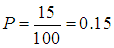
The smooth curve corresponding to the histogram in Fig. 3.2 approaches precisely the probability density as the height measurement interval is decreased.
The addition law of probabilities.
|
Two events A and B are called mutually exclusive, if they cannot occur simultaneously in a trial. |
|
The sum, (or union) of events A and B is the occurrence of at least one of them. |
The probability of occurrence of one of two mutually exclusive events A or B is determined by the addition law of probabilities:
|
|
|
(3.2) |
The generalization of law (3.2) to an arbitrary number of mutually exclusive events is obvious.
Example 1. What is the probability that an even number comes up in a single throw of a die?
Since the appearance of one of the numbers excludes the appearance of another, these events are mutually exclusive. The faces of the die carry the even numbers 2, 4, 6, whose probabilities of appearing are equal:
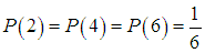
The probability of an even number coming up is
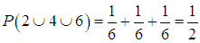
The obviousness of the result illustrates the remark of the French mathematician Laplace that probability theory is common sense reduced to mathematical calculation.
Let us again consider the group of a hundred people. Here we are dealing with the probabilities that an individual's height lies within certain limits. Thus, we know that the probability that the height lies between 175 cm and 180 cm is 0.15, the probability that the height lies between 180 cm and 185 cm is 0.10, and the probability that the height lies between 185 cm and 190 cm is 0.05. What is the probability that the height of a person chosen at random from this same group exceeds 175 cm? By the addition law of probabilities we arrive at the answer

Similarly, the probability that the height will be below 175 cm is found:

Let us now ask: what is the probability that an arbitrarily chosen individual has some height or other? This probability equals one:

which agrees with the definition of probability. We have considered an example of the probability normalization condition.
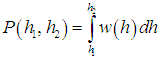
Thus, events whose outcomes take a continuous range of values are described by a continuous distribution function. For our example with the distribution of heights in a large group, we denote the distribution function by w(h). Then the infinitesimal quantity w(h)dh equals the probability that the height of an individual lies between h and h + dh. To find the probability P(h1, h2), that an individual has a height in the range

we must sum all these infinitesimal quantities, that is, calculate the area under the part of the curve w(h) between the points with coordinates h1 and h2:
|
|
|
(3.3) |
The integral of the distribution function over its entire domain must equal one, since the sum of all possible events is a certain event.
The multiplication law of probabilities.
|
The product, (or intersection), of events A and B is the simultaneous occurrence of both of them. |
|
Two events are called independent, if the occurrence of one of them does not affect the probability of occurrence of the other. |
For two independent events the multiplication law of probabilities holds:
|
|
|
(3.4) |
Example 2. Suppose two dice are thrown. What is the probability that the sum of the numbers on the faces equals 12?
This outcome is possible when sixes come up on each of the dice, and the number of points on one die obviously does not affect the number on the other. The probability sought is

Example 3. Take three groups of one hundred people each, one consisting exclusively of blondes, another of brunettes, and the third of brown-haired people. Suppose that each of them has the same height distribution as in the example considered above. Let us mix the groups and obtain a new group of three hundred people. Clearly, the height distribution has not changed under such mixing, and an individual's height does not depend on the color of his hair. The probabilities that an individual is a brunette, a blonde, or brown-haired are equal to one another and equal to 1/3. Question: what is the probability that a randomly chosen person turns out to be a brunette with a height between 175 cm and 180 cm?
The answer follows from the multiplication law of probabilities:
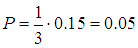
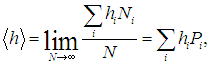
Averages. The concept of the statistical average is essentially no different from the familiar concept of the arithmetic mean and is its direct generalization. In the example under consideration we have a series of values of an individual's height. By the arithmetic mean we mean the ratio of the sum of all values of some quantity to their total number, that is, a sum of the form
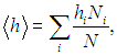
where hi — is the value of the height, Ni — is the number of individuals having this height, N — is the total number of individuals (measurements).
|
The statistical average of a quantity h, which we will denote by
|
where, by definition, Pi is the probability that the quantity h has the value hi.
For the calculation of the average height in the example considered above, we obtain
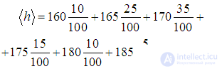
In the case of continuously distributed events, we must calculate the corresponding integral
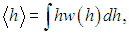
taken over the entire range of the variable h.
This section, which is central to the topic, establishes the form of the so-called Maxwell distribution.
A gas left to itself and kept under constant external conditions comes to a state of equilibrium. From the macroscopic point of view, a constant temperature and a constant pressure are established in it. If the gas consists of several components (like air, for example), then the composition of the gas will also be the same at different places in the vessel. Even in equilibrium, gas molecules move randomly, colliding with one another and with the walls of the vessel and continually changing their speeds. However, not everything is as chaotic as it seems at first glance. No matter how the speeds of individual molecules change, the mean value of the squared speed, as follows from formula (1.14) of the molecular-kinetic theory of ideal gases, remains constant and equal to
|
|
|
(3.6) |
Let us ask: how many molecules (or better, what fraction of the molecules) are moving with a definite speed (see below for what is meant by "with a definite speed") at a given moment? From the assumption of the chaotic nature of molecular motion it follows that molecules with any speeds may appear, so the distribution of molecules over speeds must be described by a continuous function. Despite the complete chaos of molecular motions, despite the random nature of collisions and of the changes in molecular speeds they cause, their distribution over speeds, as theory and experiment show, turns out to be quite definite. The nature of the speed distribution is not affected even by external fields, provided that the state of the system is one of equilibrium.
We will assume that the possible values of the speed lie in the interval from 0 to infinity. In real systems the speed cannot be infinitely large, since any system consists of a large but finite number of molecules. Therefore, even if we imagine such a practically improbable case in which all the molecules come to rest, having transferred all their energy to a single molecule, even then the energy of this molecule, and hence its speed, will be finite. We are not even speaking here of the limitations imposed by the theory of relativity, according to which the speed of any molecule cannot exceed the speed of light. Speeds that are very small and very large compared with the mean value will be regarded as possible in principle, but, as we shall see, they turn out to be improbable.
Before proceeding to consider the law of distribution of gas molecules over speeds, let us clarify the essence of the distribution problem. To determine the distribution of molecules over speeds would seem to mean to determine the number of molecules having one or another given speed. However, posed in this way the question makes no sense, since the number of molecules having an exactly (mathematically exactly!) given speed is zero. Indeed, the number of different values of the speed is infinitely large (a continuous set), whereas the number of molecules is finite. Therefore the number of molecules corresponding to each exactly specified value of the speed is zero. Consequently, the question must be formulated differently: how many molecules (or what fraction of the molecules) have speeds lying in some interval near a given speed?
Thus, to find the distribution of molecules over speeds means to determine how many molecules, or what fraction of the total number N of molecules, have speeds lying in the interval from v to v + Dv.
The distribution function of molecules over speeds. In what follows we will be concerned first of all with the probability distribution for the velocity vector  , that is, with the probability of the following event: the velocity vector
  has projections onto the axes of some Cartesian coordinate system in velocity space that simultaneously belong to the following intervals
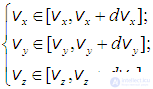
This can also be said as follows: the tip of the vector  lies inside the volume element in velocity space
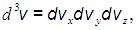
or: the vector  belongs to the volume element
  . If a spherical rather than a Cartesian coordinate system is used in velocity space, only the set of coordinates and the form of writing the volume element will change. Using a spherical coordinate system, we will have the following:
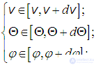
where  is the magnitude of the velocity vector, and
  and
and  are the polar and azimuthal angles characterizing the direction of the vector
  . In this case the volume element in velocity space has the form
 .
.
To shorten the notation, it is also convenient, besides the vector  , to introduce its increment
  :
:
 .
.
Here  are, as usual, the unit vectors of the Cartesian axes
 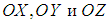 . We do not write out the corresponding expression in spherical coordinates.
Then the question posed above can also be formulated as follows: "what is the probability of the following event": the velocity vector  belongs to the (vector) interval from
  to
to 
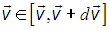 .
.
The last expression could have been written immediately; however, vectors do not form an ordered set: the question of which vector is larger,  or
or  , is meaningless, which is why the explanations above were given of what is meant by a vector belonging to some (vector) interval. A vector interval defines a volume in the corresponding space, inside which the tip of the vector lies, while the vector itself gives the position of this volume.
Differences in wording and notation do not change the essence of the matter, but they are very convenient. Nothing changes in going from an infinitesimal volume  (interval
  ) to a finite volume
  (interval
  ).
).
If DN is the number of molecules whose velocity vector, for a given state of the system, lies in the interval from  to
to  , then this number, in the general case, generally speaking, depends on:
 (interval
  );
); (since for volume elements of equal size but at different positions in velocity space, the number of particles will in general be different).
Thus,

However, it was stated and justified above that in a state of thermodynamic equilibrium the distribution of molecules over directions of motion is isotropic. In the "language" of the function  this means that it can depend only on the magnitude of the velocity vector and cannot depend on its direction.
Consequently, first,

Second, it is natural to assume that for sufficiently small volumes  , the number of molecules in it (the number of molecules whose velocity vector belongs to this volume) will be proportional to its size, that is,
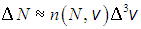
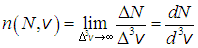
It can be shown that as the volume in velocity space  tends to zero, the approximate equality written above becomes exact. The function
  introduced above has a simple meaning: it is the concentration of particles in velocity space
Third, it seems obvious that the more particles there are in the system, the more particles, "all else being equal", there will be in the volume  and the greater their concentration
  . Therefore it is natural to go from the concentration of particles to a specific quantity that does not depend on the total number of particles in the system
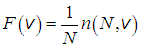
This function depends only on the speed and gives the relative number (fraction) of molecules having a velocity, per unit volume in velocity space, near a velocity of magnitude  . This function
  is called the distribution function of molecules for the velocity vector. If we take several portions of the same gas under identical conditions (the same p and T), then the distribution of molecules over speeds in them will also be identical. Knowing the form of
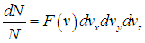
  , one can find the number of molecules dN out of the total number of molecules N, whose velocity-vector projections simultaneously belong to the intervals

This number is equal to
 ,
,
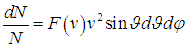
or, when spherical coordinates are used in velocity space,

Let us emphasize that this is a probability distribution for the vector of velocity, that is, for three quantities at once: either for  or for
  , depending on the coordinate system used in velocity space.
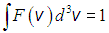
The concentration of particles in velocity space must obey a condition with a simple physical meaning: the number of molecules with all possible velocity vectors, corresponding to all the possible volumes  into which the entire velocity space can be divided, must equal the total number of particles in the system. In passing to the limit, that is, from
  to
to  , the summation turns into integration over the entire velocity space and we have:
|
|
|
(3.10) |
from which follows the normalization condition for the distribution function
 .
.
The calculation of the normalization integral written above is, of course, possible in any coordinate system in velocity space. For example, in the Cartesian system
 .
.
However, it would be a "sin" not to take advantage of the isotropy of the distribution of molecules over directions of motion, which is reflected in the dependence of the distribution function  only on the magnitude of the velocity vector. In spherical coordinates the normalization integral is considerably simpler, since two of the three integrations can be carried out in general form:

The distribution function for gases was found theoretically by Maxwell (1859) and bears his name. Below we will establish its form.
The Maxwell distribution. Since all directions of molecular motion in space are equivalent, the velocity distribution must be isotropic and the distribution function n(v) cannot depend on the direction of the velocity. This means that n(v) cannot be an arbitrary function of the velocity components vx, vy, vz, but must depend only on the absolute value of the velocity
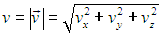
Depending on the chosen coordinate system, the probability 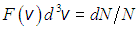 has a different form.
In the Cartesian system
|
|
|
(3.11) |
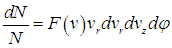
In the cylindrical system
|
|
|
(3.12) |
In the spherical system
|
|
|
(3.13) |
Next, a simple, although not entirely rigorous, derivation of the form of the distribution function is given. Consider the process of collision of two particles moving with speeds v1 and v2. Suppose that as a result of the collision the speeds of the molecules change and become vi and v4. The number of such collisions per unit time in a unit volume of gas must be proportional to the number of molecules with speeds near v1 and v2, that is, to the product n(v1)·n(v2). Let us now consider the collision process that is the reverse of this one. Here the speeds of the molecules change from the values v3 and v4 to the values v1 and v2. The number of such collisions per unit time in the volume is proportional to the number of molecules with speeds near v3 and v4, that is, n(v3)·n(v4).
By virtue of the assumption of molecular chaos and the assumption that the number of molecules with given values of speed is not changed by molecular collision processes in a gas in a stationary state, we can assume that the number of molecules whose speeds change from the values v1 and v2 to the values v3 and v4 is equal to the number of molecules whose speeds change from v3 and v4 to v1 and v2. It follows that
|
|
|
(3.14) |
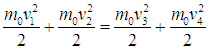
Equality (3.14) expresses the balance of particles gaining and losing the corresponding speed, and in the process of such elastic collisions the energy of the molecules is conserved (m0 is the mass of a molecule):
|
|
|
(3.15) |
Equalities (3.10), (3.14) and (3.15) constitute the set of conditions that the sought distribution function must satisfy.
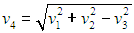
Using (3.15), let us express v4 in terms of v1, v2, v3:
|
|
|
(3.16) |
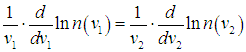
The functional equations (3.14) and (3.16) are easily converted into a simple differential equation. Taking the logarithm of (3.14), we have
|
|
|
(3.17) |
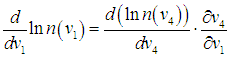
Let us differentiate (3.17) with respect to the argument v1:
|
|
|
(3.18) |
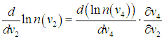
Similarly
|
|
|
(3.19) |
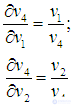
Taking expression (3.16) into account, we find
|
|
|
(3.20) |
Substituting (3.20) into the right-hand sides of relations (3.18) and (3.19), we arrive at the equality
|
|
|
(3.21) |
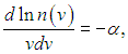
Here we must remember that this equality holds for completely arbitrary values of v1, v2, which are independent variables. This means that equality (3.21) must hold for completely arbitrary values of the speeds, so it can be satisfied only when the right- and left-hand sides of (3.21) are equal to some constant (which we denote by ( –α)):
|
|
|
(3.22) |
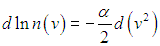
where the variable v can take the values v1, v2 or any other. Separating the variables, we write (3.22) in the form
|
|
|
(3.23) |
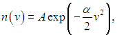
Integrating (3.23), we find
|
|
|
(3.24) |
where A — is the constant of integration. For physical reasons it is obvious that

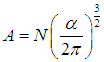
High molecular speeds are improbable. Therefore the coefficient α > 0. The constant A is determined from the normalization condition (3.10):
|
|
|
(3.25) |
It will be shown below that the parameter α must be related to the absolute temperature T by the relation
|
|
|
(3.26) |
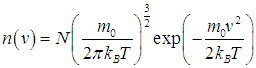
Taking (3.26) into account, from (3.24) we obtain
|
|
|
(3.27) |
Formula (3.27) is precisely the sought distribution of molecules over speeds.
Given that n(v) depends only on the magnitude of the speed and that the directions are equally probable, one can introduce the distribution function f(v) of molecules over the absolute value of the speed. To do this, expression (3.13) must be integrated over the angles, which gives
|
|
|
(3.28) |
From this and from (3.27) follows the expression for the Maxwell distribution function for the magnitude of the velocity vector f(v):
|
|
|
(3.29) |
The quantity f(v)dv is the probability of finding a particle with a speed lying in the interval from v to v + dv. The normalization condition for the distribution f(v) now takes the form
|
|
|
This section presents some consequences that follow from formulas (3.29 ) and (3.30
 ). As an example, Fig. 3.3 shows two curves corresponding to the distributions f(v) of oxygen molecules O2 over the magnitudes of speeds at temperatures T1 = 300 K and T2 = 1 300 K.
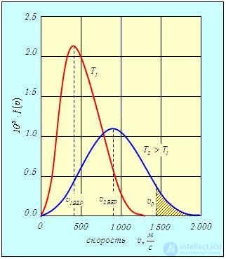
Fig. 3.3. Distribution of oxygen molecules over speeds at different temperatures T1 = 300 K and T2 = 1 300 K
The most probable speed. At infinitesimally small and unboundedly large values of speed the distribution function tends to zero

that is, such limiting values of speed are improbable in the system. Consequently, at some value of the speed the function f(v) reaches its maximum.
|
The most probable speed vmp is the speed corresponding to the maximum value of the distribution function. |
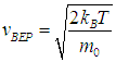
It can be found by solving the equation
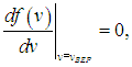
from which it follows that
|
|
|
(3.31) |
In other words, the most probable speed is the speed near which the largest number of molecules falls per unit interval. At this point f(v) takes its maximum value:
|
|
|
(3.32) |
Relations (3.31) and (3.32) can be useful for analyzing the change in the distribution function when the temperature of the gas changes or when the kind of gas, that is, the mass of the molecules, changes. Note that, as follows from (3.26) – (3.29), the Maxwell distribution depends not separately on the mass of the molecules and separately on the temperature of the gas, but on their ratio  . Therefore the distribution is the same not only "literally" but also numerically, for example, for molecular hydrogen
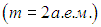 at a temperature
  and for helium
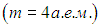 at a temperature
  .
.
As the temperature increases, the most probable speed vmp (3.31) increases, that is, the maximum of the function f(v) shifts to the right (see Fig. 3.3), T2 > T1. At the same time f(vmp) decreases, that is, the curve becomes flatter. The curve is deformed in the same way if the temperature is constant but the mass of the molecules decreases. Recall that under any deformation of the distribution function f(v) the area under the curves remains constant and equal to unity in accordance with formula (3.30).
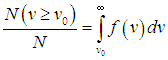
The relative number of molecules whose speed exceeds some value v0, is determined by the expression
|
|
|
(3.33) |
On the graph (see Fig. 3.3) this integral corresponds to the part of the area lying to the right of v0 (marked by hatching), bounded by the curve f(v) and the
продолжение следует...
Часть 1 3. Distribution of Molecules by Velocities and Coordinates
Часть 2 3.4. Distribution of molecules over coordinates - 3. Distribution of




 ,
,






Comments