
Lecture 52 min.
Это окончание невероятной информации про .
...
speed axis. As can be seen from Fig. 3.3, the relative number of molecules having speeds exceeding v0, increases with increasing temperature.
In conclusion of this section, let us note that all the formulas for the distribution function and the characteristic speeds contain the ratio of the mass of a molecule to the Boltzmann constant

Multiplying the numerator and denominator by the Avogadro number NA and taking into account that

— is the molar mass of the gas, and

— is the universal gas constant; we can use this relation everywhere in whichever form is most convenient for the particular problem

Distribution of molecules over dimensionless speed. If the Maxwell distribution function (3.29) is plotted with the molecular speed v, on the abscissa, the shape of the curve and the position of its maximum depend on the mass of the molecules and on the gas temperature. But if the ratio of the speed to the most probable speed is plotted on the horizontal axis, that is, the dimensionless speed

then the same curve is obtained for all temperatures and any molecular masses (any gases) (Fig. 3.4).
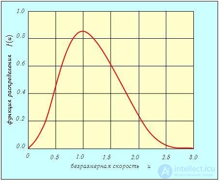
Fig. 3.4. Maxwell distribution over dimensionless speed
Making the change of variable

in (3.29 ) and taking into account that
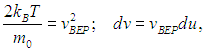
we obtain the Maxwell distribution in the form
|
|
|
(3.34) |
This formula and the corresponding graph (see Fig. 3.4) are convenient for solving many problems.
Example. Let us find what fraction of the total number of oxygen molecules at a temperature of 27 °C have speeds differing from the most probable speed by no more than 1%; and also speeds in the interval 562–572 m/s.
Let us carry out the necessary calculations. To answer the first question of the problem, note that u = 1 at v = vmp. The size of the interval is du = 0.02. Therefore,

Let us calculate the most probable speed:

Let us find the ratio of v = 562 m/s to vmp = 395 m/s
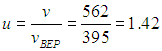
Let us determine from the curve (see Fig. 3.4) the value of the function f(u) at u = 1.42. We obtain f(u) = 0.62. The width of the interval is Dv = 10 m/s (Du = 10/395 = 0.0253). Therefore, the fraction of molecules in this interval is

It is interesting to note that an oxygen molecule travels on average a distance of 0.4 km per second. But one must not forget about molecular collisions. Because of them, a molecule moves in a straight line only for a very short time, and its path is a broken line. Therefore, a molecule moving at enormous speed along the individual segments of the broken trajectory travels from one layer of gas to another at a relatively low speed.
Mean (arithmetic average) speed. Knowing the molecular speed distribution function f(v) makes it possible to find the mean value of the speed, as well as of any quantity that is a function of speed, for example the square of the speed v2 or the kinetic energy of a molecule mv2/2.
|
The mean speed |
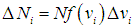
Let us divide the interval of all possible speed values from 0 to infinity into small intervals Dvi. Each interval corresponds to a number of molecules
|
|
|
(3.35) |
Since the intervals Dvi are small, we can approximately regard the speeds of the molecules in a given interval as identical and equal to vi. The sum of the speeds of the molecules in the interval is
|
|
|
(3.36) |
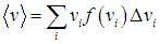
The sum of the speeds of all molecules is
|
|
|
(3.37) |
Dividing this sum by the number of molecules, we obtain the expression for the mean speed
|
|
|
(3.38) |
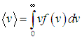
Passing from the sum to an integral, we obtain
|
|
|
(3.39) |
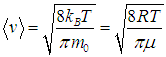
Evaluating the integral, we obtain the mean speed of the molecules
|
|
|
(3.40) |
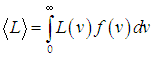
Root-mean-square speed. To find the mean value of an arbitrary function L(v) of the speed, one must multiply this function by the distribution function and integrate over all possible values of the speed:
|
|
|
(3.41) |
In particular, for L(v) = v this gives
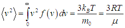
The mean value of the square of the speed equals the ratio of the sum of the squares of the speeds of all molecules of the system to the total number of molecules. Thus,
|
|
|
(3.41) |
|
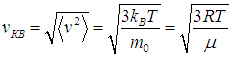
The root-mean-square speed — is the square root of the mean value of the square of the molecular speed
|
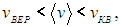
It should be noted that the characteristic speeds differ from one another only by numerical factors, and
|
|
|
(3.43) |
while their dependence on T and m0 (or m) is the same.
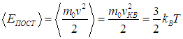
The mean kinetic energy of the translational motion of molecules is expressed through the root-mean-square speed
|
|
|
(3.44) |
This result agrees with formula (1.14) of the kinetic theory of ideal gases and with the law of equipartition of energy, which states that each degree of freedom of a molecule carries an energy of kBT/2. The three translational degrees of freedom of a molecule correspond exactly to the result (3.44) obtained here. In essence, it was precisely to obtain this agreement that we chose the coefficient α in (3.26 ) appropriately.
An experiment to test the Maxwell distribution. It must be emphasized once more that the law of the distribution of molecules over speeds established by Maxwell, and all the consequences that follow from it, hold only for a gas in equilibrium.
The law holds for any number of molecules N, provided this number is sufficiently large. Maxwell's law is statistical, and the laws of statistics are satisfied the more accurately, the larger the number of identical objects to which they are applied. For a small number of objects, significant deviations from the predicted statistics may be observed — fluctuations.
The experimental determination of the molecular speed distribution was first carried out by O. Stern in 1920. He studied the speed distribution of monatomic molecules of metal vapors (Ag or Pt) from a filament made of that metal and placed on the axis of two cylinders. The filament was heated by an electric current, and the metal evaporated (see Fig. 3.5).
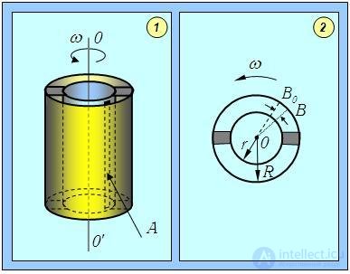
Fig. 3.5 Diagram of Stern's experiment: 1 — side view of the apparatus; 2 — top view of the apparatus
Molecules that passed through the slit in the inner cylinder flew in a straight line and settled on the wall of the cold outer cylinder. If the whole apparatus is set into rotation (with the slit always facing the point B0), then molecules with a high speed v, will land at some point near B0, while slower ones will spend more time on the way and will land at points farther from B0. Note that the emitted molecules move in a straight line; they do not take part in the rotational motion. Since molecules land at different points of the outer cylinder depending on their speed, by examining the thickness of the metal layer deposited on its wall one can form an idea of the distribution of molecules over speeds.
Let us find the distribution of molecules over the distances S from the point B0 to the place where they hit the cylinder wall. If R and r — are the radii of the large and small cylinders, respectively (see figure), then the flight time from the slit to the cylinder wall is

During this time the cylinder will turn through an angle

where ω is the angular velocity of rotation of the apparatus. Accordingly, the point of impact will be displaced relative to B0 by a distance
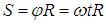
Substituting the flight time here, we obtain the relation between the speed of the molecule and the distance S:
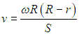
Substituting, in turn, the resulting expression into the Maxwell distribution and taking into account that

we find the distribution of molecules over the distances S:
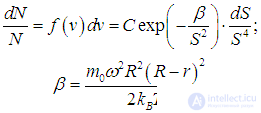
(we omit the expression for the normalization constant C).
Stern's experiments confirmed the validity of the law established by Maxwell.
In this section we turn to the analysis of the distribution of gas molecules over coordinates. Obviously, if no external forces act on the gas molecules, then in a state of thermodynamic equilibrium the gas is uniformly distributed over the given volume. In this case the pressure and density of the gas are the same at all points. If, however, the gas is in a force field (like, for example, atmospheric air, which is attracted by the Earth), then the pressure and density of the gas will no longer be the same everywhere, but will vary from point to point.
Video 3.4. Distribution of gas molecules over the height of a vessel in a uniform gravitational field.
The barometric formula. Let us find the law according to which the atmospheric pressure (or the air density) changes with distance from the Earth's surface. Let us select a vertical column of air with horizontal cross-sectional area S.
Let us assume that

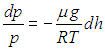
Atmospheric pressure at height h is due to the weight of the overlying layers of gas. Let the pressure at height h be p, then at height h + dh the pressure is p + dp (Fig. 3.6). Moreover, if dh > 0, then the pressure decreases, dp < 0, since the weight of the overlying layers of the atmosphere decreases.
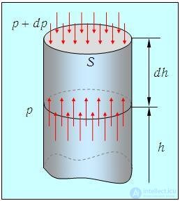
Fig. 3.6. A vertical air cylinder (for the derivation of the barometric formula)
The selected layer of gas, of height dh and mass m, is in equilibrium. Therefore, the sum of the forces acting on it is zero:

In projection onto the vertical axis we obtain
|
|
|
(3.45) |
where r is the gas density at height h. Expanding the brackets and collecting like terms, we arrive at the equation
|
|
|
(3.46) |
Let us use the Clapeyron–Mendeleev equation for the selected mass of gas m and express the density in terms of the pressure:
|
|
|
(3.47) |
Substituting (3.47) into (3.46), we finally obtain
|
|
|
(3.48) |
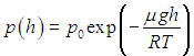
This equation can be integrated in the case of an isothermal atmosphere (T = const):
|
|
|
(3.49) |
Video 3.5. The barometric formula: a candle flame as a very sensitive indicator of the decrease of pressure with height.
The constant of integration p0 equals the pressure at the surface (h = 0). The resulting dependence is called the barometric formula. It describes the distribution of gas pressure with height in a uniform gravitational field at constant temperature. Note that the distribution depends on the kind of gas. The smaller m, the smaller the absolute value of the exponent, and the more slowly the pressure of such a gas decreases with increasing height. Figure 3.7 shows the dependence of pressure on height at temperature T = 300 K (27 °C) for three gases of different molar mass — hydrogen H2 (m1 = 2.016 g/mol), nitrogen N2 (m2 = 28.013 g/mol) and oxygen O2 (m3 = 31.999 g/mol).
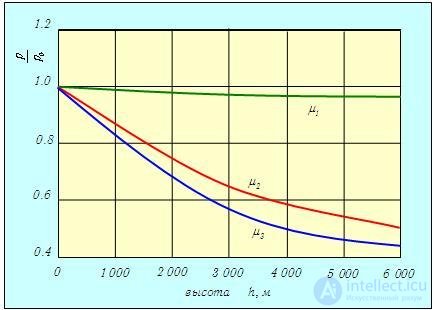
Fig. 3.7. Dependence of the pressure of three different gases H2, N2 and O2 on height
Example. Let us determine at what height the pressure of oxygen decreases by a factor of two (at T = 300 K).
We apply the barometric formula.

Then
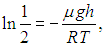
whence
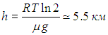
Using the ideal gas equation in the form
|
|
|
(3.50) |
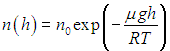
from the barometric formula one can easily obtain the law of variation with height of the number n of molecules per unit volume:
|
|
|
(3.51) |
It follows from (3.51) that the composition of air changes with increasing height: the concentration of gases with small molar mass, for example hydrogen and helium, increases.
At the surface, air is a mixture of gases: N2 — 78.08%, O2 — 20.95%, CO2 — 0.03%, inert gases — 0.94%. Let us see how the ratio of the concentrations of oxygen and nitrogen changes in an isothermal atmosphere (T = 300 K) at a height of 10 km.

The ratio of the concentrations of oxygen and nitrogen decreases from 0.27 to 0.23. Our calculation is valid only for an isothermal atmosphere and relatively small heights, for which the acceleration due to gravity changes insignificantly: g = const, T = const.
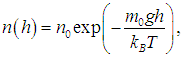
The Boltzmann distribution. The number of molecules per unit volume depends on the height h and the temperature T, and both variables enter the exponent. Equation (3.51) can be written in the form
|
|
|
(3.53) |
where kB is the mass of one gas molecule. Here the expression m0gh, in the numerator, is nothing other than the potential energy of one molecule in the Earth's gravitational field. Therefore we can say that we have a distribution of molecules over values of potential energy. The greater the potential energy, the fewer such molecules there are. In the denominator of the exponent stands kBT — a quantity proportional to the mean energy of the thermal motion of a molecule. The higher the temperature, that is, the greater the energy of the thermal motion of the molecules, the more slowly the exponential factor, which is proportional to the concentration of molecules, decreases with height. Figure 3.8 shows curves of the relative concentration of oxygen molecules O2 at different heights for two different temperatures T1 = 300 K and T2 = 1 300 K (the latter case is, of course, unrealistic and is used merely as an illustration).
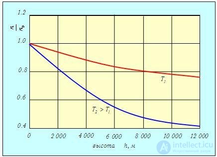
Fig. 3.8. Dependence of the relative concentration of oxygen molecules on height at different temperatures T1 = 300 K and T2 = 1 300 K
We see that at a higher temperature the number of particles per unit volume decreases more slowly with height. As the temperature decreases, most of the particles are located at lower heights. And at T = 0 all the particles would be located on the Earth's surface. This fact has a simple physical explanation. Each particular distribution of molecules over height is established as the result of two competing tendencies:
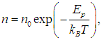
Denoting Ep = m0gh, we obtain
|
|
|
(3.53) |
that is, the concentration of molecules is greater where their potential energy is smaller. Particles are more likely to be found at those points of space where the potential energy is lower.
Boltzmann showed that such a distribution holds in the field of any forces, not only in a gravitational field. Therefore the distribution (3.53), where n — is the concentration of particles with potential energy Ep is called the Boltzmann distribution.
We have established the function describing the distribution of molecules over speeds (the Maxwell distribution) and the relation characterizing the distribution of molecules over values of potential energy (the Boltzmann distribution). Both relations can be combined into a single generalized distribution.
Consider an infinitesimal volume dV of gas located at the point with position vector  in a large system representing an ideal gas at constant temperature in external force fields. The number of molecules in the selected volume is n(
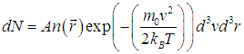
  ) d3r. Since the volume is small, the particle density within it can be considered constant. This means that the condition for the validity of the Maxwell distribution is satisfied. Then, by combining relations (3.11) and (3.27), we obtain the following formula for the number of molecules dN with speeds from v to v + dv located in the volume d3r :
|
|
|
(3.54) |
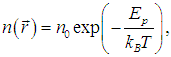
But the concentration of molecules n(r) depends on the location of this volume in the external force fields:
|
|
|
(3.55) |
where n0 — is the concentration of molecules at the point where Ep = 0. Then
|
|
|
(3.56) |
Since the expression
|
|
|
(3.57) |
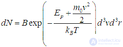
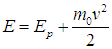
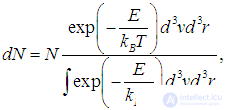
represents the total energy of a particle in an external potential force field, we arrive at the generalized Maxwell–Boltzmann distribution over the energies of molecules:
|
|
|
(3.58) |
where N — is the total number of particles in the system, and dN — is the number of particles with coordinates between r and r + dr and (simultaneously) with speeds between v and v + dv.
Mean energy of a quantum oscillator. The Maxwell–Boltzmann distribution was obtained in classical physics, but it turned out to be valid in quantum mechanics as well, where many seemingly unshakable propositions were subjected to revision. As an example, consider the problem of a load of mass m, attached to the end of a spring of stiffness k. The equation of motion is well known, and its solution is harmonic oscillation of the body with angular frequency

The classical energy of the system, which models the vibrations of atoms in a molecule, is given by formula (3.62) and can take any value depending on the amplitude of the oscillations. As we know from quantum mechanics, the vibrational energy is quantized, that is, it takes a discrete series of values determined by the formula:
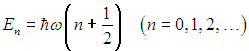
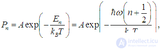
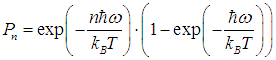
In accordance with the general principles of statistical physics, the probability Pn of finding the oscillator in a state characterized by some value n of the vibrational quantum number is determined by the formula
|
|
|
(1) |
where A — is the normalization constant. To determine it, one must use the probability normalization condition
|
|
|
(2) |
To do so, into the well-known formula for a geometric progression
let us substitute the value
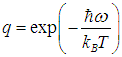
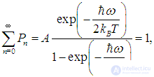
We then obtain, instead of (2)
|
|
|
(3) |
|
|
|
(4) |
from which the expression for the constant A follows. Using it in expression (1), we arrive at the probability
|
|
|
(5) |
We see that the larger the value of the quantum number n, the lower the probability of finding the oscillator in such a state. The higher the temperature, the larger the values of n that become practically significant for the system. As

all probabilities Pn with n > 1 tend to zero, and only

In other words, at zero temperature there are no thermal excitations, and the oscillator performs "zero-point oscillations" — it is in the ground state with the lowest energy

The distribution of oscillators over energies as a function of the temperature of the system is shown in Fig. 3.9
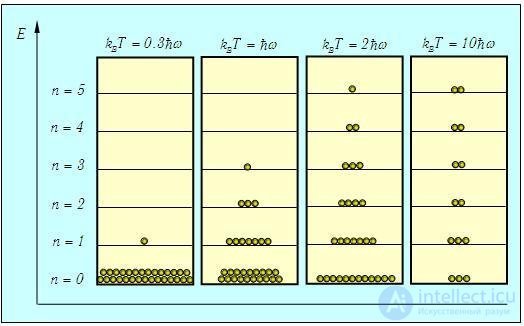
Fig. 3.9. Approximate distribution of N = 30 quantum oscillators over energy levels as a function of temperature. Only the ground state and the first five excited energy levels are shown. At T = 0 all oscillators are in the ground state. As the temperature rises, higher and higher energies become accessible, and the distribution of oscillators over levels becomes more and more uniform
For clarity we have taken a system with a small number (N = 30) of oscillators (strictly speaking, statistical laws apply to systems with a much larger number of particles).
The question arises: what is the mean value
|
|
|
(6) |
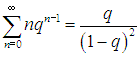
To do this, let us differentiate with respect to q both sides of equality (3.67) for the geometric progression:
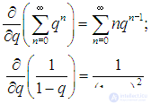
from which we obtain
|
|
|
(7) |
Using (7) at
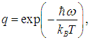
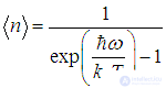
we obtain from (6) the expression for the desired average
|
|
|
(8) |
Now it is easy to obtain the average energy of the oscillator
|
|
|
(9) |
where the function cth — the hyperbolic cotangent is defined by the relation
|
|
|
(10) |
In Fig. 3.10 the solid line shows the average energy of a quantum oscillator, measured in units of ħω,
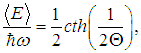
as a function of the "dimensionless temperature"

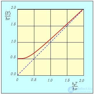
Fig. 3.10. Average energy of a quantum oscillator as a function of temperature
The dashed line

corresponds to the result of classical physics. Indeed, the energy

per degree of freedom is the average value of both the kinetic and the potential energy of a classical oscillator, so that the average value of the total energy is exactly

We see that quantum corrections are important at low temperatures: for q < 0.3 the average energy of the oscillator is close to the ground-state energy ħω/2. In this case one says that the vibrational degrees of freedom are "frozen out," that is, the thermal energy is insufficient to excite vibrations. But already at q = 2 the two energies practically coincide, that is, the quantum corrections are small. The value q = 1 can be taken as a conventional boundary between the quantum and classical regions. Its meaning is transparent: at

the thermal energy equals the minimum excitation energy of the oscillator, that is, the difference between the energy

of the first excited state and the energy

of the ground state of the oscillator.
What temperatures can be considered low for an oscillator that models a real system, for example a hydrogen molecule H2? The characteristic frequencies of molecular vibrations usually lie in the infrared region and are of the order of ν = 1014 Hz. This corresponds to the energy

and the temperature
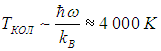
Average energy of a quantum rotator. Thus, the room temperatures familiar to us turn out to be quite low from the point of view of exciting molecular vibrations. Let us see what happens to molecules at temperatures T < Tvib. Since there are no vibrations, a diatomic molecule can be represented as a "dumbbell" — two atoms rigidly connected to each other. Such a system is called a rotator and, as we saw earlier, has five degrees of freedom — three translational (motion of the center of mass) and two rotational. The energy of rotational motion of a classical rotator has the form (3.61). Taking into account the relation

between the angular frequency of rotation ω, the moment of inertia I and the angular momentum L, we write the classical rotational energy of the molecule as

In quantum mechanics the square of the angular momentum is quantized,

Here J is the rotational quantum number, so the energy of rotational motion of the molecule is quantized as well
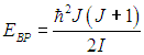
Using this relation and the Maxwell–Boltzmann distribution, one can obtain an expression for the average energy of a quantum rotator. However, in this case the formulas are rather complicated, and we will restrict ourselves to qualitative results. At high temperatures the average energy tends to the classical value kBT, corresponding to two degrees of freedom (rotation about two orthogonal axes). At low temperatures the rotator will be in the ground state, corresponding to J = 0 (no rotation). The "transition" between these two limiting cases evidently occurs at a temperature Trot at which thermal motion is able to excite the rotational degrees of freedom. The minimum (nonzero) rotational energy is equal to

as follows from the formula for Erot at J = 1. Therefore
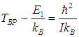
For the moment of inertia of the molecule we can adopt the estimate

where mp = 1.67·10–27 kg (the proton mass), and aB = 5·10–11 m is the Bohr radius. We then obtain
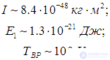
The resulting estimates are confirmed by measurements of the molar heat capacity at constant volume cnV, which we already discussed in the previous chapter. At temperatures below 100 K only the translational degrees of freedom of the molecule take part in thermal motion. The average energy of a molecule is 3kBT/2, and the energy of one mole is 3NAkBT/2=3RT/2, whence the heat capacity is cnV = 3R/2. In the temperature range from 100 K to 200 K the molar heat capacity increases to the value cnV = 5R/2, which indicates the "unfreezing" of two additional (rotational) degrees of freedom (that is, the addition of kBT of energy per molecule). In the region of temperatures from 4,000 K to 5,000 K the molar heat capacity increases again, this time to the value cnV = 7R/2. This is the "unfreezing" of the vibrational degree of freedom, which brought an additional energy kBT per molecule.
Rate of chemical reactions. Chemists have an empirical rule that when the temperature rises by 10 °C the reaction rate doubles. This is merely a rough generalization, and there are many exceptions to it, but on the whole it is more or less true. An explanation can be given here too, on the basis of the Maxwell–Boltzmann distribution.
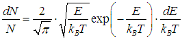
For many chemical reactions to proceed, the energy of the particles involved must exceed a certain threshold value, which we denote E0. The more such particles there are, the higher the reaction rate. The distribution of particles over energies follows from formulas (3.28), (3.29). One only has to express the particle speed v in terms of its kinetic energy E

and take into account that

As a result we obtain the distribution of particles over energies
|
|
|
(11) |
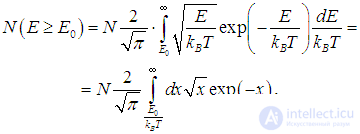
From this we find the number of particles with energy E > E0:
|
|
|
(12) |
where we changed the integration variables

For numerical estimates we take the threshold energy equal to the molecular vibration excitation energy: E0 = 6·10–20 J. Then for room temperature T1 = 300 K we obtain E0/kBT1 = 14.5, and for the temperature T2 = 310 K this ratio is E0/kBT2 = 14.0. The numbers of particles participating in the reaction are determined by the relations
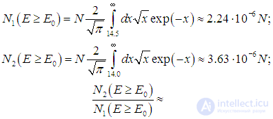
Indeed, raising the temperature by only 10 degrees led to a 60% increase in the number of particles whose energy exceeds the threshold value.
Часть 1 3. Distribution of Molecules by Velocities and Coordinates
Часть 2 3.4. Distribution of molecules over coordinates - 3. Distribution of













Comments