4. Transport Phenomena: Laws and Theory

In the previous chapters we dealt with equilibrium systems. As a result of the motion of molecules and the redistribution of energy among them, equilibrium temperature and particle concentration are established in the various parts of the system. For example, in the absence of external fields the particle concentration will be the same in all parts of a system in equilibrium. In an external gravitational field the particle concentration varies with height, but has a strictly definite value and is the same in the horizontal direction.

In real systems, however, situations arise in which the system is not in equilibrium. A difference (a gradient, in scientific language) of temperature, particle concentration, density, or momentum can arise between parts of the system. Then fluxes of the corresponding quantity arise in the system in the direction opposite to its gradient, so that the system approaches a state of thermodynamic equilibrium. Processes of this kind are called transport phenomena; as we shall see in this chapter, they are responsible for the thermal conductivity of bodies, the viscosity of fluids, and the diffusion of particles (Fig. 4.1). Here we continue to use the molecular-kinetic approach. Our goal is to understand how wandering molecules carry various physical quantities to other parts of the system.

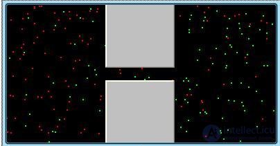
Fig. 4.1. Model of diffusion of particles through an opening

4.1. Molecular collisions

In discussing the ideal gas, we proceeded from the assumption that molecules do not interact with one another. In fact, of course, what was assumed was the absence of potential energy of interaction between them. Elastic collisions between molecules, and between molecules and the walls, must necessarily occur, if only because otherwise there would be no mechanism by which an equal distribution of energy over the degrees of freedom is established, and otherwise one could not speak of the temperature of the system, the pressure in it, and so on. Collisions of molecules occur at random. They change the direction and magnitude of the particles' velocities, but do not change the distribution of molecules over velocities and coordinates in equilibrium systems.

A question arises: will molecules always collide with one another? After all, molecules are very small, and the distances between them in an ideal gas are an order of magnitude greater than their linear dimensions. Perhaps in vessels of small size they fly from wall to wall without collisions? Let us calculate how many times per unit time one molecule can collide with others and what distance it travels on average between collisions.

Before proceeding to the calculations, let us adopt the simplest model for molecules. We will represent them as elastic balls. In a collision of molecules with effective diameters d₁ and d₂ their centers approach to a distance (d₁ + d₂)/2 (Fig. 4.2).

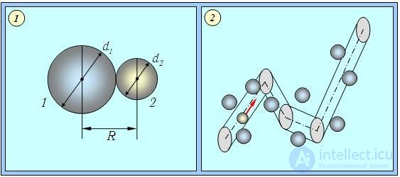
Fig. 4.2. Collision of two molecules (1) and the trajectory of a selected gas molecule (2): its direction of motion changes when some molecule of the medium falls within the interaction radius R = (d_t + d₂)/2

If we imagine that molecule 1 runs into molecule 2, a collision will occur if the first molecule falls within a sphere of radius

circumscribed around the second molecule. The cross-sectional area of this sphere is

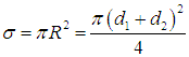
The quantity R is called the effective interaction radius of molecules 1 and 2, and — the effective interaction cross section of these molecules. In a collision of identical molecules d₁ = d₂ = d, R = d and

In the time between two successive collisions a molecule travels some path l. Of course, for each individual molecule it is a matter of pure chance how far it manages to advance without collisions. But averaging the path l over all molecules of the system, we obtain the physical quantity

called the mean free path of the molecules. The statistical meaning of this quantity is as follows: the ratio of a small segment of length dx to gives the probability of a collision

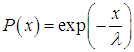
on the path dx. Let P(x) — be the probability of traveling a distance x without collisions. Then

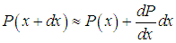
— is the probability of traveling a distance x + dx without collisions. The latter event is made up of two independent events:

the particle traveled a distance x without collisions (the probability of which is P(x));

the particle also traveled the additional small segment of path dx without collisions (the probability of which is 1 – dx/). By the multiplication theorem for probabilities we then have

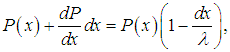
whence follows the equation for the probability P(x)

Since the probability of traveling zero distance without collisions is equal to unity, we additionally have the initial condition P(0) = 1. Integrating the differential equation, we finally find

As we can see, the greater the path x, the smaller the probability of traveling it without collisions.

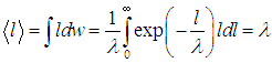
Let us now verify that — is indeed the mean free path. Let us calculate the probability that a molecule will have free path length l. This means that the particle traveled a distance x = l without collisions (the probability of which is P(l)) and collided with another particle immediately after that — on a small segment of length dl (the probability of which can be found as dl/). By the multiplication theorem for probabilities, the probability dw of such an event is equal to

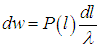
We then find the mean free path

Of course, one should not think that the probability of traveling a distance l without collisions is zero: some of the molecules may travel very large distances, but only an extremely small fraction of them. For x = , as follows from (4.1), the probability of traveling without collisions is

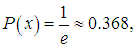
that is, 63.2% of the particles will experience collisions on this path. For a path length x = 2 we obtain

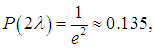
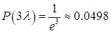
that is, 86.5% of the particles are already fated to collide, and at x = 3 as many as 95% of the particles take part in collisions, since

To determine the average number of collisions n of one molecule with others per unit time, we make the following assumptions:

• all molecules are identical, that is, we do not consider mixtures of gases;
• all molecules except the one we are observing are at rest (later we will show how to get rid of this obviously incorrect assumption);
• in collisions the speed v_rel of the molecule does not change (this assumption is, in essence, of the same level as the previous one: in an elastic collision with an obstacle that remains at rest, the magnitude of the velocity indeed does not change (the meaning of the subscript "rel" will become clear later)).

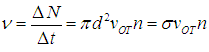
The path of our molecule of diameter d remains straight until it meets a stationary molecule whose center lies at a distance from the line of motion smaller than R = d. After that the molecule changes its direction of motion and moves in a straight line until the next collision. During the time interval ∆t the molecule travels a broken path v_rel ∆t and collides with all molecules that fall within a broken cylinder of radius d and base area = πd ² (see Fig. 4.1). The volume of this cylinder is πd ² v_rel ∆t. If n is the concentration of molecules in the system (their number per unit volume), it is easy to find the number of stationary molecules in the cylinder, that is, the number of collisions ΔN:

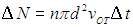
From this follows the collision frequency (that is, the number of collisions per unit time)

Let us now get rid of the consequences of our assumption that the molecules are at rest. Suppose we are following molecule 1, which moves with velocity v₁, and it collides with molecule 2, which has velocity v₂. In the reference frame attached to the second molecule, it is at rest, whereas the first molecule has velocity

It is now clear that it is precisely the average value of the relative velocity of the molecules that plays the role of the speed v_rel used by us in deriving relation (4.3) for the collision frequency. We then have

where 𝜃₁₂ is the angle between the directions of motion of the molecules. Because of the randomness of the motion, this angle takes any values with equal probability, so that the average value of its cosine is zero. And averaging the squares of the velocities leads to the appearance of the root-mean-square speed of the molecules

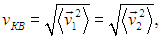
familiar to us from the previous chapter. We finally obtain that

and formula (4.3) is written in its final form

Note that, by passing from the speed of the molecule to its root-mean-square speed, we have in fact also got rid of the third assumption, since v_rms is constant at a given temperature.

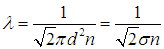
Knowing the collision frequency, we can find the mean free path. Indeed, the average time between two successive collisions is = 1/n, and during this time the particle travels on average a path = vrmst. Thus, the mean free path of a gas molecule is equal to

Since at constant temperature the particle concentration is proportional to the pressure, the mean free path decreases as the pressure increases. This is understandable, since the average distance between particles decreases. In reality a molecule is not a hard ball. Therefore its effective diameter d is not quite constant: it decreases as the temperature increases, although only slightly. Hence the mean free path grows slightly with increasing temperature.

It should be noted that the average distance between particles is far from coinciding with the mean free path. Earlier we estimated the effective diameter of a water vapor molecule as d = 3·10^{–10 m} and the average distance between molecules under normal conditions as L = 3·10^–9 m. From this we find the concentration of molecules

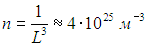
Substituting the found n into the expression for the mean free path, we find

We see that the mean free path is 200 times the diameter of the molecule and 20 times the average distance between molecules. For completeness let us also estimate the collision frequency. The kinetic energy of translational motion of a molecule is

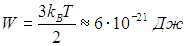
Knowing the mass of a water molecule

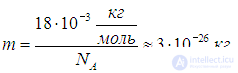
we obtain an estimate of the root-mean-square speed

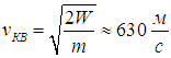
Finally, we determine

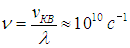
In other words, a molecule experiences 10 billion collisions per second! The linear size of a vessel containing one liter of gas is l = 10 cm = 0.1 m. At a speed of 630 m/s the molecule could travel from wall to wall in a time

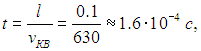
but during this time it will experience

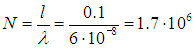
collisions with other molecules.

We have left undiscussed the first assumption, that all molecules are identical. It was needed not for reasons of principle, but to simplify the derivation and the final expressions. If this is not so, if we consider a mixture of gases, then the components have different particle concentrations and different root-mean-square speeds, and their molecules have different masses. As a consequence, the formula for the mean free path will change, and the results will differ for molecules of different kinds.

Example. Let us find how formula (4.6) for the mean free path changes if the molecules are flat disks moving in the material of a thin film, unable to escape from it.

As before, for molecules of diameters d₁ and d₂ to collide, they must approach to a distance

Therefore, as a molecule moves in the plane of the film, it will hit all other molecules that fall within a broken rectangle (in contrast to the cylinder in the three-dimensional case) of width 2R and length v_rel ∆t. The area of this rectangle is

With a surface concentration n of molecules (in this case n is their number per unit area), ∆N = Sn collisions will occur. From this we find for the collision frequency

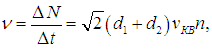
where we took into account that, as before, the relative velocity

From this the mean free path for flat molecules moving in a plane is found to be

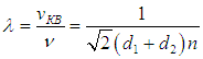
For identical molecules (d₁ = d₂ = d)

A date in the forest, a hedgehog in the fog, and an atomic bomb. The idea of the mean free path can be used to estimate visibility in a forest, in fog, or even to roughly estimate the critical mass of uranium in an atomic bomb.

Imagine that you have a date in a forest. From what maximum distance R will you notice your partner (and your partner, you)? Suppose you turn on a flashlight to signal to him or her. If we ignore light scattering, then all the trees cast shadows whose linear size can be taken to be approximately equal to the tree diameter d. In Fig. 4.3 your location is marked by a red circle, a circle of radius R, is drawn around it, the trees are shown as green circles, and their shadows on the circle are marked by orange arcs.

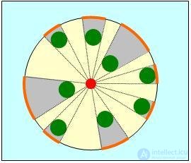
Fig. 4.3. Estimating the maximum visibility distance R in a forest

Let us determine what part of the circle is covered by shadows. Let n be the density of tree planting (their number per unit area). If l is the average distance between trees, then

Inside the circle there are pR²n trees. The total length of the shadow on the circle is therefore pR²nd. We see that the total shadow length grows as the square of the radius and at some value of R will exceed the circumference 2pR. But if the whole circle is covered by shadows, light cannot pass any farther. This value of R will be the maximum visibility distance in the forest. It is now clear that it is determined from the equality

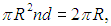
that is, we have obtained the estimate

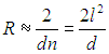
For a numerical example we can take values from everyday experience. Say a rendezvous is arranged among birch trees with an average trunk diameter d = 0.25 m and an average distance between trees l = 10 m. Then we find R = 800 m.

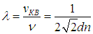
Let us now relate the result obtained to the formula for the mean free path. Here one molecule (the light ray) has no size (d₁ = 0), the size of the other molecules equals the average trunk diameter (d₂ = d), and finally the molecules (the trunks) are at rest, so the factor must be dropped. As a result, for our problem, we obtain the expression

Thus the visibility radius we found is

The probability that light travels this distance without "collisions" with trees is

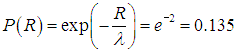
In other words, with a probability of 86.5 % the light will be stopped by the trees.

The rendezvous in the forest took place in a plane. Now we return to the three-dimensional world. The same figure now shows a sphere of radius R and obstacles in the form of little balls of diameter d. For example, we want to estimate visibility for a hedgehog lost in fog, and the role of the trees is now played by water droplets. If the concentration of droplets is n (their number per unit volume), then inside the sphere there are

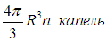
Their shadows on the sphere are circles of area pd²/4. At the maximum visibility distance the shadows cover the entire sphere:

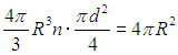
From this we find the visibility distance in fog

Let us again compare this result with formula (4.6) for the mean free path of a molecule in a gas, where the factor must be dropped and we must take

We obtain

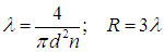
The probability of traveling the path R = 3l without collisions is

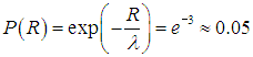
Consequently, with a probability of 95 % a collision will occur on this path.

Let us obtain a numerical estimate. Our reasoning is valid if the droplet size noticeably exceeds (say, by one or two orders of magnitude) the wavelength of light. Since the visible range has wavelengths 0.40–0.76 μm, for the droplet diameter we adopt the estimate d = 10^–4 m. For the droplet concentration we take the value n = 3·10⁷ m^–3 (for the origin of this number see just below). Then the visibility in fog will be

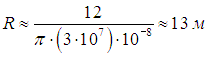
We estimated the droplet concentration as follows. The saturated water vapor pressure at, say, 20 °C (T = 293 K) is p_s = 2.3·10³ Pa. Applying the Clapeyron–Mendeleev equation, we find the density of water vapor at 100 % humidity:

With a sharp drop in temperature all the vapor condenses into droplets of the indicated size, forming a dense fog. The mass of one droplet is

The number of droplets formed in a volume V is found as the ratio of the vapor mass m to the droplet mass m_drop. Then the droplet concentration is determined from the relation

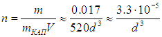
For d = 10^–4 m we obtain the value used above, n = 3·10^–7 m^–3.

The dependence of the visibility distance in fog on the droplet size is thus given by the relation

For extremely small droplets with a diameter of about ten light wavelengths, d = 10^–5 m, the visibility shrinks to one meter. As the saying goes, "you can't see beyond your own nose." For still smaller droplets our model becomes invalid, since light can no longer be treated simply as a collection of particles of negligibly small size. Diffraction effects begin to play a role, and the expression for the effective cross section for the interaction of light with the droplets is no longer determined purely by the geometric cross section of the droplets.

The problem solved here also bears on the critical mass of uranium-235 used to make atomic bombs. Instead of light we have neutrons in this problem, and instead of droplets, ²³⁵U nuclei. In collisions with nuclei, neutrons split them into fragments, and 3–4 more neutrons are emitted. At the critical radius R_cr the number of neutrons will not decrease and a self-sustaining chain reaction will arise — an atomic explosion will occur. As a basis for determining the critical radius we can take the visibility radius

reduced by a factor of k (k = 3.5 is the neutron multiplication factor). Since

we obtain

The nuclear radius is

where r₀ = 1.4·10^-15 m is the radius of a nucleus with mass number A = 1, that is, of a proton (neutron). Therefore the effective interaction diameter is

From a reference book (for example, the Russian Encyclopedic Dictionary) we find the density of uranium r_U = 19·10³ kg/m³. The mass of a uranium-235 nucleus is determined from the proton mass

From this we find the nuclear concentration

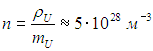
Now we can estimate the critical radius R_cr

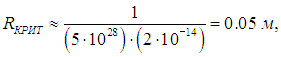
the critical volume V_cr

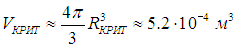
and the critical mass M_cr

Note that we are giving away no secrets of nuclear weapons production: these estimates are far too crude. Our only aim is to demonstrate once again the unity of the laws of physics operating in the most diverse systems.

4.2. Laws of transport processes

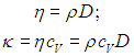
If a gas is driven out of equilibrium, processes arise in it that tend to return the system to equilibrium. For example, different parts of the system have different temperatures or particle concentrations. Accordingly, the temperatures or concentrations tend to even out (owing to the thermal motion of molecules), which is accompanied by the transfer (transport) of certain physical quantities from one part of the system to another. Such processes are called transport phenomena. These phenomena have much in common and are classified according to which physical characteristic is "transported" from one part of the system to another.

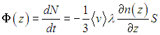
Diffusion. Suppose the system contains molecules whose concentration n(z) depends on the coordinate z. Let us mentally place at the point with coordinate z a small square of area S, perpendicular to the z axis. In the system a process of equalization of the concentration n of particles takes place, accompanied by their transport in the direction of decreasing n. Experiment shows that through the area S in unit time there passes a number of particles

where D is determined by the properties of the system and is called the diffusion coefficient. The quantity Φ (the particle flux — the number of particles per unit time) has dimension

the dimension of the particle concentration is

and therefore the dimension of the diffusion coefficient is

The negative sign in the law of diffusion means precisely that the particle flux is directed from larger concentration values to smaller ones, that is, in the direction opposite to the derivative dn/dz. Indeed, let n(z) — be a decreasing function, that is, the particle concentration falls with increasing z. Then the derivative dn/dz (the concentration gradient ) is negative, and the flux Φ turns out to be positive, that is, directed toward increasing z.

If both sides of equation (4.7) are multiplied by the mass m₀ of the diffusing molecules, then for the mass flux M = m₀Φ we obtain the analogous equation

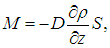
where r = m₀n — is the mass of the diffusing substance per unit volume, that is, its density. The relation (4.7) between the particle flux and the concentration gradient dn/dz is called Fick's first law.

Fick's first law says nothing about the value of the diffusion coefficient, which in each specific case must be determined experimentally. Therefore this law is empirical in nature. It applies not only to gases but also to solids and liquids. It should also be noted that the transport of matter in gases and liquids can also occur mechanically, through convection currents (say, by wind in the atmosphere or a current in the ocean). It is important not to confuse diffusion, which occurs because of molecular motion, with convection, which arises from the action of external forces.

Note that if the system is a mixture, then Fick's first law is written in exactly the same form for each component of the mixture separately, but the diffusion coefficients, generally speaking, differ. This means that in a mixture of, say, two gases it may happen that the particle concentration of one component has already equalized while that of the other has not yet.

Fick's second law makes it possible to find the dependence of the concentration of diffusing particles on time. To derive it, consider two identical small squares parallel to each other, located at nearby points with coordinates z and z + dz. For definiteness we assume that n(z) — is a decreasing function (Fig. 4.4).

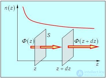
Fig. 4.4. Illustration of the phenomenon of diffusion (for the derivation of Fick's second law)

Then through the left area, in time dt there enter Φ(z)dt particles, and through the right one there leave Φ(z + dz)dt particles.

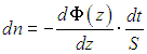
The increase in the number of particles dN in the space between the areas in time dt equals the difference between the numbers of entering and leaving particles:

Dividing dN by the volume Sdz of the gap between the squares, we obtain the change in particle concentration in time dt

Using Fick's first law, we find from this (here we already switch to partial derivatives)

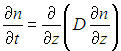
Usually the diffusion coefficient does not depend on the coordinates, and we obtain the equation expressing Fick's second law:

If we introduce the particle flux density j = Φ/S (the number of particles crossing a unit area per unit time), then equation (4.8) can be written in a different form:

This equation is one example of a continuity equation, which appears in many areas of physics and here expresses the law of conservation of the number of particles. Its meaning: the rate of change of the number of particles in a volume equals the difference between the fluxes of entering and leaving particles (provided that no particles are created or destroyed inside the volume).

Viscosity. Consider the following thought experiment. Let a plate float on the surface of a liquid, slowly pulled to the right with a force F_T (Fig. 4.3).

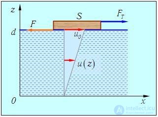
Fig. 4.5. The internal friction force F, acting on a plate, moving with speed u₀ over the surface of a liquid

Experiment shows that in steady motion the plate moves with a constant speed u₀. Let the distance to the stationary bottom be d, and the area of the plate be S. What can we say about the flow of the liquid?

It is clear that besides the force F_T something else must act on the plate: otherwise it would move with uniform acceleration. This "something else" can act only from the liquid. In other words, a force F, similar to a friction force, acts on the plate from the liquid. It is directed to the left and equals in magnitude the applied force F_T. What is the origin of this force? The layer of liquid adjacent to the plate "sticks" to it and moves with the same speed u₀. Similarly, the layer of liquid adjacent to the bottom has zero velocity. Consequently, a certain velocity distribution u(z), is established in the system, where z — is the distance from the bottom. Ultimately the stationary bottom acts on the plate through the liquid, giving rise to the internal friction force, already familiar to us from the mechanics of liquids and gases.

Video 4.2. The internal friction force in a gas: an experiment with disks.

In accordance with the above, the boundary conditions u(0) = 0, u(d) = u₀ must certainly hold. The internal friction force arises precisely because of this velocity distribution: an overlying layer "rubs" against the underlying one and is slowed by it (correspondingly, the faster layer tends to accelerate the slower one).

Experiment shows that the internal friction force F is related to the speed u₀ by the relation (see Fig. 4.3)

The coefficient h, which has dimension

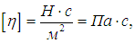
is called the coefficient of dynamic viscosity (internal friction).

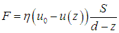
To find the velocity distribution in this system, imagine an observer located at a distance z from the bottom and moving together with the liquid with speed u(z). From this observer's point of view, his layer is at rest, and the plate moves with speed u₀ – u(z). The dependence of the same force F on speed must now be described by an analogous formula with the replacement

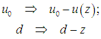
As a result we obtain

Equating expressions (4.11) and (4.12), we find the speed of the layer as a function of distance from the bottom

We have obtained a linear law of velocity distribution (Fig. 4.6), satisfying our boundary conditions u(0) = 0, u(d) = u₀.

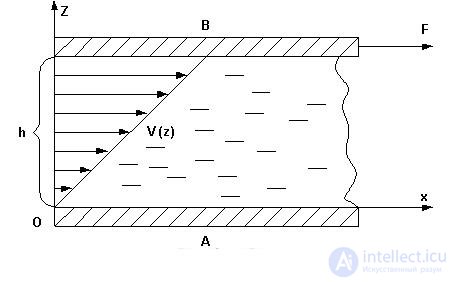
Fig. 4.6 Linear velocity distribution in a liquid

Such a velocity distribution is due to the simplicity of the system considered. In other cases the flow is more complicated, but even then we can make use of the relation found. Indeed, consider a liquid in which there is a velocity gradient along the coordinate z. The relative velocity of layers with coordinates z and z + dz is

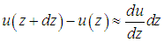
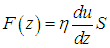
Since we are considering arbitrarily small distances dz, for small areas S the flow can be regarded as planar and described by the previous formulas. Then the internal friction force between adjacent layers will be determined by equation (4.11), where in place of the ratio u₀/d stands the velocity gradient of the relative motion of the layers du/dz:

Such a law indeed corresponds to experiments determining the internal friction force between layers of a liquid or gas in laminar flow, and was established by Newton.

Thermal conduction. Suppose now that there are two heat sources of different temperatures T₁ and T₂. Imagine them as wide plates arranged perpendicular to the z axis at the points with coordinates z = 0 and z = d. The gas filling the gap between the plates transfers thermal energy from the hot body to the colder one. In this process a certain temperature distribution T(z), is established in the gas, satisfying the boundary conditions T(0) = T₁ and T(d) = T₂ (Fig. 4.).

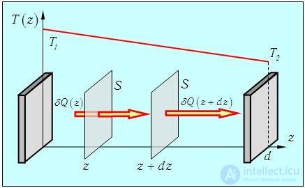
Fig. 4.7. Temperature distribution between two sources

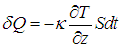
Let us place between the sources a small square of area S, parallel to the plates. Experiment shows that in time dt an amount of heat dQ, flows through the area S, and

The constant k is called the thermal conductivity and has dimension

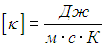
Relation (4.15) is called Fourier's law.

The negative sign (as in Fick's first law) indicates that the heat flux is directed toward decreasing temperature, that is, against the temperature gradient dT/dz. Under these conditions a linear law of temperature variation will be established in the gas in the equilibrium state. Indeed, through a small square of unit area located at the point z, the following amount of heat flows in per unit time

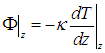
Through an identical square at the point z + dz the following heat flows out per unit time

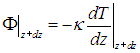
If the temperature between the squares does not change (equilibrium has been established), then these heat fluxes are equal to each other, that is,

From the vanishing of the second derivative it follows that the function is linear:

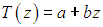
From the boundary conditions at the end points we find the integration constants:

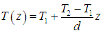
In essence, we have obtained an analog of the velocity distribution law found in considering the viscosity of a liquid: it suffices to make the replacement

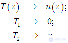
This is a consequence of stationarity, that is, of the fact that we considered a steady flow or temperature distribution. The same follows from Fick's second law: for a stationary system the time derivative on the left-hand side of equation (4.9) is zero, whence it follows that the second derivative of the particle concentration with respect to the coordinate z, is zero, which is equivalent to the linearity of the function n(z).

Example. Let us determine how much thermal energy is carried away per unit time through a window of area S = 2 m² with a distance between panes d = 5 cm, if the room is kept at temperature t₁ = 20 °C, while outside it is freezing:
t₂ = –20 °C.

Note at once that since the size of a degree on the Celsius and Kelvin scales is the same, the temperature difference is

The thermal conductivity of air is k = 0.025 J/(m·s·K). For glass this coefficient is 20 times larger, so its presence can be neglected. Besides, the thickness of the glass is much less than the gap between the panes. Therefore it is precisely the air layer between the panes that protects us from the frost. In accordance with the above, a linear temperature distribution is established in this gap, so that the derivative dT/dz is constant and equal to

The thermal energy flux is then

The consumption of thermal energy through one window in a month is

In solving this problem we implicitly made a strong assumption: that the temperature of the inner pane coincides with the room temperature, and that of the outer pane with the temperature of the surrounding air. From experience everyone knows this is not so: in reality the outer surface of the glass is somewhat warmer, and the inner one somewhat colder. In fact the temperature gradient in the gap between the frames may be about half as large, which correspondingly reduces the outward flux of thermal energy. However, an exact solution of the problem is beyond the scope of this course.

It is easy to notice what all the phenomena discussed have in common. Every transport equation contains the gradient of some quantity — particle concentration, flow velocity, temperature. In all cases, under stationary conditions a linear distribution of this quantity is established. All this is because transport phenomena have a common origin — molecular motion.

4.3. Kinetic theory of transport

The laws stated above describing transport phenomena — Fick's first law and the analogous laws for internal friction and thermal conduction — were established experimentally. In this section we shall show that they follow from the molecular kinetic theory. The basis of all transport phenomena is the chaotic motion of molecules. On moving to other parts of the system, molecules carry there information about the conditions in which they previously found themselves. Transport of mass (or the very passage of particles) is characteristic of diffusion. Transfer of energy from some layers of gas to others constitutes the essence of thermal conduction. And, as we shall see, transfer of momentum underlies the phenomenon of internal (molecular) friction in a gas or liquid.

Diffusion. Let us first analyze the process of diffusion (more precisely, self-diffusion, that is, diffusion of somehow-labeled molecules in a medium consisting of identical particles). In this case the mean speeds of the particles of the medium and of the diffusing particles are the same, and the mean free path is given by the already familiar expression

Let us mentally select in the medium some area S and direct the z axis perpendicular to it. The other two axes x and y are parallel to the area. We model the chaotic motion of the molecules as follows. We assume that exactly 1/3 of the molecules move along the axis x, 1/3 along the axis y and 1/3 along the axis z. Of the molecules flying parallel to z, exactly half (1/6 of the total number of molecules) move in the positive direction, and the same number in the negative direction. Let us count the number of molecules crossing the area S per unit time (Fig. 4.8).

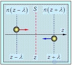
Fig. 4.8. Counterflows of particles through the area S from regions with different particle concentrations (for the derivation of Fick's first law)

It is clear that molecules flying along the x and y axes will not cross the area. In time dt molecules cover the distance dt. Therefore only 1/6 of the molecules from the volume dtS on the right and 1/6 of the molecules from the same volume on the left will reach the area. But the particle concentrations on the left and on the right are different (n depends on z).

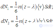
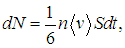
An attentive reader may ask: we fix an infinitesimal time interval dt, and therefore the volumes under consideration are disks of infinitesimal thickness dt. So it would seem that the particle concentrations on the left and on the right should coincide. The question is a fair one, but the point is that the last time before reaching the area S, the molecules collided with other molecules at a distance of one mean free path l from the area. Therefore, they approach the chosen area with the particle concentrations n(z – l) and n(z + l), which have been established at the points with coordinates z – l and z + l, respectively (z is the coordinate of the area). The number of particles reaching the area from the left is dN₁, and from the right, dN₂, and these numbers will differ:

(4.16)

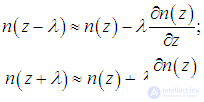
Since l is small, we can expand the particle concentrations in a series, keeping only the first two terms:

(4.17)

The total number of particles dN, crossing the area in the positive direction of the z axis, equals the difference between the numbers of particles crossing the area from the left and from the right. We then find

(4.18)

The expression for the particle flux

(4.19)

has exactly the same structure as Fick's first law (4.7). Thus, we have not only derived this law but also determined the diffusion coefficient:

(4.20)

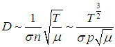
Taking into account that

and that

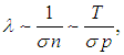
(4.21)

This dependence of the diffusion coefficient in gases on temperature and pressure is confirmed by experiment.

Viscosity. Let us now consider the mechanism by which gas viscosity arises. We will now imagine the z axis as vertical, in accordance with Fig. 4.9.

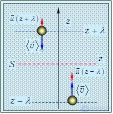
Fig. 4.9. Counter-flows of particles through the area S from regions with different velocities of ordered particle motion (for the derivation of the viscosity law)

Let us now assume that the particle concentration is the same in all parts of the system, so that the numbers of particles

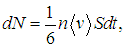
arriving from below and from above are equal. However, the molecules come from layers with different velocities of ordered (not molecular!) motion u(z). When a slower molecule from the lower layer enters the upper layer, it slows down the ordered motion of that layer, while itself being accelerated. Conversely, molecules from the upper layer accelerate the lower layer and are slowed down by it. Thus, this process tends to equalize the velocities in the system, and this is precisely what the phenomenon of internal friction (viscosity) consists of.

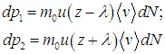
We assume that the velocity of ordered motion is much smaller than the mean velocity of thermal motion of the molecules (which is hundreds of meters per second). Then the mean velocity of thermal motion can still be considered constant. For the momenta of ordered motion transported through the area S from below and from above, we have

(4.22)

From this, for the total momentum transported in the positive direction of the z axis, we obtain

(4.23)

In this formula we used the gas density

The transported momentum is parallel to the velocity u, and its direction depends on the sign of the derivative. For the velocity distribution shown in Fig. 4.3, the velocity increases with increasing z, so that the derivative

The minus sign in equation (4.23) means that the momentum arriving from below from the slower layers is smaller than the momentum arriving from above from the faster layers. Therefore, the momentum of the layer with coordinate z tends in this case to increase by the amount –dp. The derivative

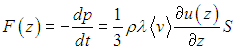
gives the force acting on the fluid layer of area S with coordinate z

(4.24)

We have derived law (4.14) and obtained an expression for the coefficient of dynamic viscosity

(4.25)

It is now easy to establish the dependence of the coefficient of dynamic viscosity on temperature and the type of gas:

(4.26)

Note that the coefficient of dynamic viscosity ultimately does not depend on the density, that is, on the pressure. This is because as the pressure increases, the gas density increases, but the particle concentration grows proportionally, that is, the mean free path decreases. These two factors compensate each other.

Thermal conductivity. Let us now analyze the phenomenon of thermal conductivity. Suppose that the particle concentration is the same everywhere in the system, so that the same number of particles crosses the area from the left and from the right, as in the consideration of diffusion:

(4.27)

so that the total particle flux through the area S (Fig. 4.10, compare with Fig. 4.8) is zero.

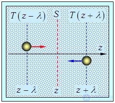
Fig. 4.10. Counter-flows of particles through the area S from regions with different gas temperatures (for the derivation of the thermal conductivity law)

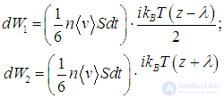
However, the molecules bring with them the mean energies w, which they had in the layers with coordinates z – l and z + l. These energies are proportional to temperature:

Multiplying the mean energy by the number of particles crossing the area, we obtain for the amount of energy transported by them from the left and from the right

(4.28)

For the heat transported in the positive direction of the z axis, we obtain from this the expression

(4.29)

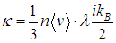
We have derived law (4.15) and found the coefficient of thermal conductivity

(4.30)

Video 4.3. Thermal conductivity of gases. Butane – air at equal and different pressures.

Recall that i is the effective number that determines the mean energy of a molecule. Since

the coefficient of thermal conductivity does not depend on the molecule concentration or the gas density. Its dependence on temperature T and the type of gas is as follows:

(4.31)

Video 4.4. Thermal conductivity of gases. Neon – air at equal pressure.

Video 4.5. Thermal conductivity of gases. Air – air at different pressures.

Let us introduce the specific heat capacity of the gas at constant volume

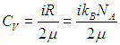
and take into account further that the mass of a molecule is

from which the relation between the particle concentration and the gas density follows

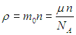
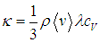
Then we obtain a somewhat different expression for the coefficient of thermal conductivity:

(4.32)

The analysis above yields formulas relating the corresponding transport coefficients (see relations (4.20), (4.25) and (4.32)):

(4.33)

Let us give numerical estimates, using the results obtained earlier for water vapor, which are typical of all gases under normal conditions: density

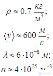
Then we find the diffusion coefficient

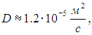
the thermal conductivity (i = 6 for water vapor)

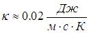
and the dynamic viscosity

Let us compare the estimates obtained with experimental data for air:

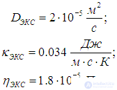
We see that we have not gone wrong, at least in the orders of magnitude, even though our estimates of the coefficients are not quite accurate.

4.4. Brownian motion

The problem of the wandering sailor. Let us first solve the classic problem of the drunken sailor. A sailor leaves a tavern and sets out to walk home. He moves with constant speed v but is able to maintain the chosen direction of motion only over a path length l, that is, for a time

After that he is turned around, loses his bearings, and moves in some other direction. The choice of direction each time is random, so that all directions are equally probable. The question is: at what average distance R_T from the tavern will the sailor be at time t (it is assumed that ). The word "average" here means the following. Suppose that this happens every day, and each time we measure the sailor's distance from the tavern. The root mean square of the values obtained over a large number of trials (say, over a year) gives us the desired quantity R_T.

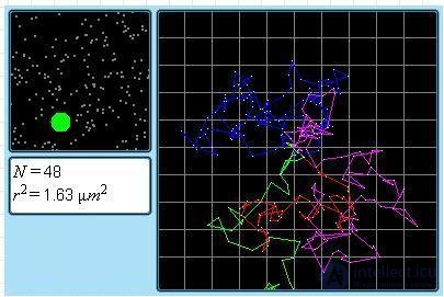
Fig. 4.11. Model of Brownian motion

Video 4.6. Physical model of Brownian motion.

So, let us take the tavern as the origin of coordinates and characterize the sailor's position at time by the position vector R. The sailor's path consists of straight segments, whose number is k = t/. Let i be the segment number (i = 1, 2, ..., k). We specify the sailor's displacement along segment number i by the vector r_i, so that for all values of i we have (Fig. 4.12)

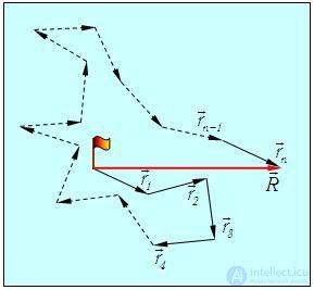
Fig. 4.12. Trajectory of the wandering sailor

Then the position vector R is represented as the sum of the vectors r_i

Let us square both sides of equality (4.34):

Here — is the angle between the vectors r_i and r_j. Let us now average both sides of equality (4.35) over all instances of the sailor's walk from the tavern. The average values of all the cosines are zero because the sailor's choice of the next direction of motion after a straight segment is equally probable in all directions. We then obtain

From this follows the desired root-mean-square distance

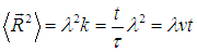
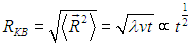
Note that this distance depends on the square root of time, in contrast to the case of rectilinear, uniform motion. This substantially changes the character of the motion. Let us give a numerical example. Suppose the sailor moves slowly, with speed v = 0.9 km/h = 0.25 m/s. In a time t = 3 h = 10,800 s, moving in a straight line, he would have gone a distance of 0.9·3 = 2.7 km. Suppose that he is able to move in a straight line only = 10 m. Then his average distance from the tavern over the same time will be

Brownian motion and diffusion. Leaving our sailor to meander in the vicinity of the tavern, we may ask: what does he have to do with the molecular kinetic theory? It turns out, the most direct connection. Suppose a dust particle floats in water, and we observe it through a microscope. The particle is subjected to impacts from the molecules of the medium, randomly changing its direction of motion and speed.

The randomness of the particle's trajectory here is due to the fact that:

• a different number of molecules may strike it from different sides
• molecules striking from one side may at that moment have higher speeds than molecules striking from the other.

Therefore, the particle moves along a broken-line trajectory. This phenomenon is called Brownian motion. As the temperature increases, the intensity of Brownian motion grows. As the size of the particle increases, the randomness of its collisions with molecules is smoothed out, and Brownian motion becomes unobservable. Brownian motion is the most direct proof of the chaotic nature of molecular motion. Our wandering sailor is a simulation of Brownian motion. With this simple problem we have demonstrated a characteristic feature — the dependence of the root-mean-square displacement of the particle on the square root of the time of motion. The product in equation (4.43) has the same dimensions and the same structure as the diffusion coefficient. Therefore, for Brownian motion as well, we should expect a dependence of the root-mean-square displacement of the form

Brownian motion is closely related to diffusion. Let us turn to Fick's second law (4.9). This is a first-order equation in time, and it allows us to find the function n(z, t) if the initial particle concentration n(z, 0) is given. We will not solve this problem exactly. We only note that with the passage of time the initial distribution "spreads" in space and at the same time changes its shape. But there is one type of distribution — the Gaussian, or normal distribution, — whose shape remains unchanged with time (it only "spreads"). We will deal only with this simplest case, which nevertheless allows us to obtain all the characteristic features of the process. For the calculations we will need two standard integrals:

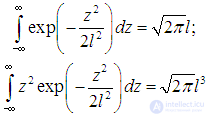
Let the distribution of particle concentration at the initial time t = 0 have the form

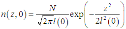
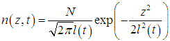
The form of this function is shown in Fig. 4.13

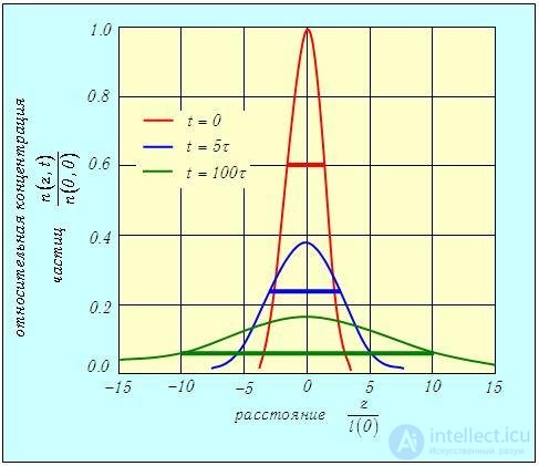
Fig. 4.13. Spreading of the Gaussian distribution of particle concentration with time: the three curves correspond to three different values of time, measured in units of t = l²(0)/(2D); the abscissa shows "dimensionless" distances, measured in units of the half-width l(0) of the initial distribution; the ordinate shows the ratio of the particle concentration n(z, t) to its maximum value n(0, 0) at the initial time t = 0; the horizontal segments show the root-mean-square width 2l(t)/l(0) of each of the distributions

Video 4.7. "Generation" of a Gaussian distribution using millet grains.

Here N — is the total number of particles distributed along the z axis with concentration n(z, 0):

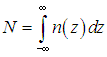
The quantity l(0) characterizes the width of the distribution. Indeed, the expression

gives the relative number of particles in the interval (z, z + dz), that is, the probability that a particle is found in this interval. Therefore, the mean value of the squared coordinate is

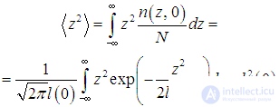
If we define the width of the distribution as the distance between the points

and

then

is the root-mean-square half-width of the distribution at the initial time t = 0.

As already mentioned, the Gaussian distribution is the only one that does not change its shape as it spreads. This means that at an arbitrary time t the distribution will have the form

Correspondingly, for an arbitrary time

where the as yet unknown function l(t) is the changing half-width of the distribution.

Our task has become simpler: instead of solving the partial differential equation (4.9), it is now enough to substitute (1) into it, verify that it is indeed a solution, and find the time dependence of the half-width of the distribution, that is, determine the function l(t).

Let us differentiate (1) with respect to the coordinate z:

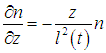
Let us differentiate (1) with respect to z once more, taking into account the result of the first differentiation:

Now let us differentiate (1) with respect to time:

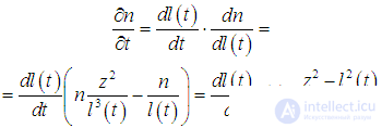
Substituting expressions (2) and (3) into equation (4.9) of Fick's second law, we verify that n(z, t) in the form (4.46) is indeed its solution, provided the half-width of the distribution l(t) satisfies the equation

This equation is easily integrated:

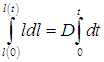
or

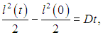
from which we find the time dependence of the half-width of the distribution:

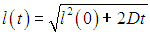
If at the initial time t = 0 all the molecules were concentrated at a single place (l(0) = 0), then

which reproduces, at a new level, the result we guessed when analyzing the sailor's wanderings. The increase in the half-width of the distribution gives the displacement of the Brownian particle. The expression for the root-mean-square displacement of a Brownian particle

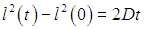
is the classic Einstein–Smoluchowski result; they constructed the theory of Brownian motion.

Example. A female student enters the lecture hall. Let us estimate the time after which the smell of her perfume reaches the examiner sitting at the table.

We estimated the diffusion coefficient of molecules in gases as

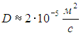
Let us take the distance l(t) to the examiner to be 4 m, and the width of the initial distribution is approximately equal to the diameter of the student's head, l(0) = 0.2 m. Since l(t) >> l(0), we can use equation (4.52), from which we find

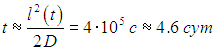
The answer is clearly absurd and contradicts all the world's experience of administering exams. It is clear from this example that the spreading of smells through a room occurs not by diffusion but through faster processes. It turns out that our nose can respond to a mere handful of molecules, so to sense a smell it is enough for just a few of the fastest molecules from the "tail" of the Maxwell distribution to reach the examiner's nose. Plus, of course, convection: the door opened by the student creates an air flow that carries the perfume molecules fast enough.

Numerical estimates for Brownian motion. If diffusion processes are so slow, how was it possible to observe Brownian motion? To answer this question, we will now estimate the diffusion coefficient of a dust particle in a liquid. We already know that the square of the root-mean-square displacement of a particle along some axis depends linearly on time:

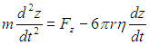
This law can be used to determine the diffusion coefficient of Brownian particles. Let us now consider the equation of motion of a particle along the chosen axis z:

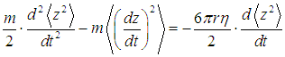
Here F_z — is the random force acting on the particles from the molecules, and the second term on the right-hand side — is the force resisting the motion of the particle due to the viscosity of the liquid according to Stokes' law (it is assumed that the Brownian particles are spheres of radius r). Since we are interested in the time dependence of the square of the coordinate z, we multiply equation (2) by z and use the relations

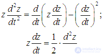
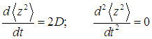
Averaging the resulting equation, we arrive at the expression

Here it is taken into account that z> = 0 owing to the randomness of the forces acting on the dust particle from the molecules. By virtue of (1)

Substituting these values into (3) and taking into account that

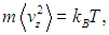
we find the desired expression for the diffusion coefficient of Brownian particles

Let us now carry out numerical estimates. The radius of the Brownian particles (dust particles) is r = 0.5·10^–6 m. Taking h = 10^–3 Pa·s (water) and T = 300 K, we obtain from (4)

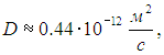
which is much smaller than the diffusion coefficient of the student's perfume molecules from the example considered above. Nevertheless, Brownian motion is observable. For instance, in 30 s the root-mean-square displacement of the particle will be

which is five times the diameter of the dust particle. Therefore, such displacements can be observed under a microscope. The example demonstrates a well-known scientific truth: quantities in themselves cannot be considered small or large a priori; everything is understood by comparison.