
Lecture
Solving the identification problem includes a stage of formalizing the object of study [6, 9, 33]. Depending on the stated goal, the type of model, methods, and identification algorithms are determined.
Modern hydromechanical units (HMU) of engine control systems (ECS) for aircraft engines (DLA) include a wide variety of design solutions; therefore, taking into account the general design features of HMU ECS DLA, it is expedient to consider the formalization of an industrial pump-regulator as an example.
Formalizing the pump-regulator as a typical representative of hydromechanical units makes it possible to define the range of models inherent to this class of objects and to demonstrate the use of identification methods and algorithms.
The main purpose of the pump-regulator is automatic control of fuel supply to the engine combustion chamber and control of the compressor and turbine geometry, based on commands from the primary and backup automation [25].
The functional diagram of the pump-regulator is shown in Fig. 3.2.
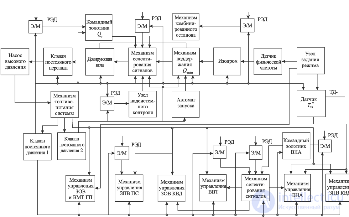
Fig. 3.2. Functional diagram of the pump-regulator
Within the automatic control system, the pump-regulator performs the following functions:
• fuel supply to the combustion chamber and to the working cavities of the engine's power elements; regulation of fuel flow to the combustion chamber based on an electronic signal from the primary automation (PA) control system — the engine's electronic controller;
• control of the high-pressure compressor (HPC) rotor speed depending on the position of the engine control lever αcl
and the inlet air temperature Tin* over the
"idle – maximum" and "idle – full reverse" ranges when operating on backup automation (BA) upon PA failure;
• metering of fuel supply during startup as a function Qf = f (τ), with manual correction provided on BA upon PA failure,
where Qf is the metered fuel flow rate to the combustion chamber and τ is time;
• ensuring the minimum fuel flow rate Qmin in the "idle" mode on BA upon PA failure;
• metering of fuel supply during acceleration and deceleration
as a function Qf = f (τ) on BA upon PA failure;
• controlling the position of the air bleed valves (ABV) from the intermediate HPC stages depending on the corrected
HPC rotor speed nHPCcorr;
• controlling the position of the high-pressure compressor's inlet guide vane (IGV) blades based on an electronic signal from the electronic engine controller, and, upon PA failure, from the BA control system, depending on nHPCcorr;
• together with the engine's hydraulic cylinders, ensuring repositioning of the air bleed shutters downstream of the booster stages (ABS BS) based on an electronic signal from the PA, and, upon PA failure, ensuring the open position of the shutters via the BA system;
• together with the engine's hydraulic cylinders, ensuring repositioning of the air-to-air heat exchanger (AAHE) shutters for turbine blade cooling and the shutter for air bleed used to cool the turbine casing, based on an electronic signal from the PA, and, upon PA failure, ensuring "AAHE shutters open" and "casing-cooling air-bleed shutter closed" from the BA;
135
• together with the engine's hydraulic cylinders, ensuring control of the repositioning of the shutters for air bleed used to cool the turbine casings and the shutter for air bleed used to cool the compressor casing, based on an electronic signal from the PA control system, and, upon PA failure, the shutters must be controlled by the BA using the HPC ABV control signals;
• together with the engine's hydraulic cylinders, ensuring control of the air-oil heat exchanger (AOHE) shutter of the hydraulic drive (HD) and the air bleed shutter (ABS) for anti-icing of the air intake, depending on the HPC rotor speed;
• ensuring the transition of engine control to the BA upon
the HPC rotor speed or the air pressure PK* downstream of the HPC reaching extremely high values while operating on the PA;
• ensuring engine shutdown.
In accordance with the functions listed above, the following basic hydraulic units/subsystems can be identified within the pump-regulator (see Fig. 3.2):
• high-pressure pump;
• constant-pressure valve;
• all-mode speed governor;
• engine operating-mode setting unit;
• actuating element of the inlet air temperature sensor at the
engine inlet;
• physical speed sensor;
• start-up automatic device;
• minimum fuel flow maintenance mechanism;
• fuel-supply mechanism for the units' automation system and control of the power elements of the engine's variable geometry mechanisms;
• signal selection mechanism;
• supersystem monitoring unit;
• combined engine shutdown mechanism;
• mechanism for controlling the IGV and HPC ABS when operating on backup automation;
• mechanism for controlling the position of the ABS and the hydraulic-drive AOHE shutter;
• unit for controlling the air bleed shutters downstream of the booster stages;
136
• mechanism for controlling the hydraulic cylinders of the air bleed shutters used for cooling the turbine and compressor casings;
• mechanism for controlling the AAHE shutters;
• unit for controlling fuel flow based on signals from the primary automation;
• unit for controlling the IGV based on signals from the primary automation. Thus, the pump-regulator represents a complex,
multiply-connected hydromechanical system consisting of nineteen subsystems.
3.2.1. Selecting the type of mathematical model for the industrial pump-regulator
The identification problem for the pump-regulator can be solved using methods of structural or parametric identification [3, 6, 7, 9]. The parametric identification problem consists in estimating the model parameters from observations of the input and output variables obtained under the object's operating conditions. In this case, the structure of the object (the class, type, and dimensionality of the model) is known. The structural identification problem requires the prior solution of problems such as selecting the model's structure and class, and evaluating the object's stationarity and linearity, among others.
As noted above, the choice of model structure is based on the purpose of studying the object and on the intended further use of the model.
For describing the hydromechanical units of aircraft engine control systems, it is expedient to use parametric identification methods, since the structure of the object is known a priori and is determined by the unit's design.
Constructing a full-scale model of the pump-regulator is complex and impractical; therefore, it is proposed to apply the principle of functional decomposition of the system by functional attribute. The functional breakdown of the system presented above can be considered sufficient for the formal implementation of this principle.
Another aspect of this problem is the choice of a method for the mathematical description of the object. Among the best-known and most widely used approaches, the following methods of mathematically describing hydromechanical systems should be noted [25]:
137
• sensitivity models;
• factor models;
• linearized models;
• element-by-element models.
Sensitivity models are the simplest, but are applicable only to linear systems. The nonlinearity of the characteristics of many hydraulic-system elements does not allow a reliable model of the HMU ECS DLA to be obtained.
The construction of factor models is based on the apparatus of design-of-experiment methods. The factors chosen are the variables that determine the operating mode and the adjustment elements. The main drawback of factor models is that the identification algorithm becomes more complex as the number of factors grows. Like the sensitivity model, the factor model is not multi-mode.
Unlike factor models and sensitivity models, linearized dynamic models of HMUs reflect the physical structure of the object. However, a linearized model is reliable only for small deviations from the linearization point, so linearized models are unsuitable for modeling an HMU "at large" (over a wide operating range).
The most accurate way of mathematically describing hydromechanical systems is the element-by-element model [34, 35], which represents the statics and dynamics of hydraulic systems over the entire range of coordinate variation, with the model's coordinates coinciding with the physical coordinates of the object.
3.2.1.1. Constructing element-by-element models
An element-by-element model is a way of describing hydraulic systems in which each element of the hydraulic circuit is described
using the basic equations of dynamics [34, 35]:
• the equation of balance of forces applied to the moving elements of hydraulic systems:
∑Fi (x) +∑Fi (u) = M
d 2 x
;
(3.1)
2
i
i
dt
• the moment-balance equations:
138
∑Ri(θ)+∑Ri(u)= J
d 2θ
;
dt
2
i
i
• the flow-balance equations:
∑Q1i −∑Q2i = dV
+V dP,
i
i
dt
B dt
(3.2)
(3.3)
where u, x are the input and internal dynamic variables (coordinates); Fi (x), Ri (θ) are forces that are functions of the linear coordinates x and the angular coordinates θ; Fi (u), Ri (u) are forces that are functions of external parameters (input signal, pressure disturbance,
flow rate,
rotational speed, etc.);
M
is the mass
of the
element
under consideration;
J is the moment of inertia; Qi , Qi
are the incoming and outgoing
1
2
flow rates;
V
is the volume of liquid in the element; P is the pressure of the liquid
in the element;
B is the bulk
modulus of
elasticity;
dV
is the change in
dt
volume over time; VB dPdt is the change in volume due to the compressibility
of the liquid.
Based on an analysis of the forces acting in hydraulic systems, the following can be identified:
• elastic forces:
Fi (x) =Ti +ci x,
(3.4)
where Ti
is the initial tension; ci
is the stiffness of the elastic link;
• friction forces:
F (x) = − f
dx,
(3.5)
i
i
dt
where fi
is the friction coefficient;
• forces depending on external parameters:
Fi (u) =Ti′+ Kiu,
(3.6)
where Ti′
is the initial value of the force; Ki
is the proportionality
coefficient;
139
• pressure forces:
Fi (u) = Si Pi ,
(3.7)
where Si is the surface area; Pi
is the pressure.
Taking into account the forces (3.4)–(3.7), the balance equation (3.1) takes the form
∑Ti +∑Ti′+∑Kiu +∑ci x +∑Si Pi + dx∑fi = M d 22x.
(3.8)
i
i
i
i
i
dt i
dt
Equation (3.8), after moving the origin of coordinates to the point of static equilibrium and replacing the stiffness of the elastic link with the equivalent stiffness ci = −ci [34], takes the form
∑Kiu +∑Si Pi = ∑ci x + dx∑fi + M d 22x.
(3.9)
i
i
i
dt i
dt
Similarly, for the moment equation:
′
dθ
∑ϕi + J
d 2θ
,
(3.10)
∑Kiu = ∑ciθ+
dt
dt
2
i
i
i
where K′ is the proportionality coefficient; ci is the equivalent stiffness of the elastic link; ϕi is the friction coefficient.
In the flow-balance equation (3.3), the incoming and outgoing flow rates are determined by the flow capacity of the jets, throttle packs, and throttling orifices:
Q = S
2
∆P,
(3.11)
ξρ
where S is the equivalent cross-sectional area; ξ is the drag coefficient; ρ is the density of the working fluid; ∆P is the pressure drop across the throttle or jet.
Analysis of the terms in equations (3.1)–(3.3) showed that the power of the useful signal is significantly greater than the power lost to friction and to overcoming the inertia of moving masses; the deformation of the hydraulic system's walls is negligible compared to the volume of liquid in the system; the compressibility of the liquid practically
has no effect on the operation of the system. Consequently, when constructing a model of hydraulic units, the following factors can be neglected: the forces of viscous and dry friction; the inertia of moving masses; the compressibility of the liquid, and the deformation of the hydraulic system's walls. Taking these assumptions into account, the element-by-element model of the hydraulic system's elements takes the form
∑Kiu +∑Si Pi =∑ci x,
i
i
i
′
∑ i
∑
i
u =
(3.12)
K
c θ,
i
i
2
(∑S1i
P − P1 −∑S2i
P2 )= S dxdt ,
ξρ
i
i
where
S
is the surface area of the movable elements of the hydraulic systems;
Si , Si
are the areas of the inlet and outlet orifices; P is the constant
1
2
working pressure;
P1
is
the pressure downstream of
the inlet orifice; P2 is
the pressure upstream of the outlet orifice.
It can be seen from the system of equations (3.12) that the dynamic coordinates in the HMU model are the displacements of the hydraulic system's movable elements. All other variables are related to them by algebraic equations. Selecting the displacements of the movable elements as the dynamic coordinates is reasonable, since they are the output parameters of the hydraulic system's dynamic functional elements. Moreover, displacements are, for the most part, measurable quantities in hydraulic systems.
For the further identification procedure, the element-by-element model (3.12) needs to be formalized, i.e., presented in vector-matrix form (state space). Such formalization is impossible because of the presence of nonlinear operations such as products and exponentiation; therefore, to formalize the models in terms of state space, classical linearization methods are applied to the element-by-element model [25, 34]:
141
∑Kiu0 +∑Ki∆u +∑S0i P0i +∑∆Si P0i +∑S0i∆Pi =
i
i
i
i
i
= ∑ci∆x +∑ci x0 ,
i
′
i
′
(3.13)
∑Kiu0
+∑K ∆u = ∑ci∆θ+∑ci∆θ0 ,
i
i
i
i
2
Si
∑S10i
P − P10 −∑
10
∆P1 +∑∆S1i P − P10 −
P − P
ξρ i
i
i
10
Si
dx
−
Si
− ∆Si
P
−
20
∆P
P
= S
.
∑
∑
20
20
2
∑
2
20
dt
i
i
Р20
i
The subscript "0" denotes the value of the parameter at the linearization point.
After moving the origin of coordinates to the linearization point and solving the system of linearized equations with respect to the dynamic coordinates by the variable-elimination method, the system of equations (3.13) takes the form
∑K
∆u +
∑∆S P
+ ∑S
∆P =
∑c ∆x,
i
i
i
i 0i
i
0i
i
i
i
′
∑c
∆θ,
∑K
∆u =
i
i
i
i
2
Si
i
Si
(3.14)
−∑
10
∆P
+ ∑∆S
P − P
−∑
20
∆P
−
ξρ
i
P − P10
i
i
P20
P
)
= S dx.
−∑∆Si
i
2
20
dt
The dynamic coordinates in the hydraulic system are the displacements of the movable elements, and the dynamic equations are the flow-balance equations. After solving the system of equations (3.14) with respect to displacement, it takes the form
dx
= a∆x +b∆u ,
(3.15)
dt
where a = f1(u0 ,P0 ,x0 ,S0 ,S10i ,S20i ,P10i ,P20i ), b = f2 (u0 ,P0 ,x0 ,S0 ,S10i ,S20i ,P10i ,P20i ).
142
The formalized model (3.15) serves as the basis for solving the identification problem.
Thus, the procedure for constructing a formalized element-by-element model consists of three stages.
1. Describing each element of the hydraulic system using the basic equations of dynamics:
∑K
u
+∑S P
= ∑c x,
i
i
i
i i
i
i
'
= ∑ciθ,
∑Kiu
i
i
2
∑Si
P
− P
−∑Si
ξρ(
i 1
1
i
2
2. Linearizing the system of equations:
∑K
∆u +
∑∆S P
+ ∑S
∆P
=
∑c
∆x,
i
i
i
i 0i
i
0i
i
i
i
'
∆u = ∑c
∆θ,
∑K
i
i
i
i
2
Si
−∑
10
∆P +
∑∆Si
P − P
ξρ
i
P − P10
i
P
)
= S dx.
−∑∆Si
i
2
20
dt
P2 )= S dxdt.
Si
−∑
20
∆P −
2
i
P20
3. Reducing the system to a formalized form: dxdt = a∆x +b∆u.
3.2.1.2. Mathematical models of the functional elements of the pump-regulator
The functional decomposition of the pump-regulator presented earlier made it possible to identify nineteen subsystems, comprising limiting elements, relay-type elements, and dynamic links that provide analog control of the aircraft engine control system's subsystems. From the standpoint of constructing mathematical
143
models, the dynamic links are of particular interest, and they include [25]:
• the all-mode speed governor, which includes a constant-pressure-drop valve (CPDV) and an isodrome regulator;
• the actuating element of the inlet air temperature sensor at the
engine inlet;
• the physical speed sensor;
• the start-up automatic device, the Qmin maintenance mechanism;
• the mechanism for controlling the IGV and HPC ABS on backup automation;
• the Qf control unit based on signals from the primary automation;
• the IGV control unit based on signals from the primary automation.
As an example, the mathematical description of the speed governor is given below. The hydraulic diagram of the engine shaft speed governor is shown in Fig. 3.3.
Functionally, the speed governor consists of:
• a physical speed sensor (loop I);
• an isodrome regulator (loop II);
• a constant-pressure-drop valve, which controls the position of the swash plate of the pumping unit (loop III).
The physical speed sensor serves to enable operation of the all-mode governor controlling the speed of the high-pressure compressor rotor. The sensor's hydraulic diagram is shown in Fig. 3.3 (loop I) and consists of a centrifugal speed sensor, a pendulum 2 with springs, a hydraulic amplifier 3 with a feedback lever 4, and a servo piston 5.
The mathematical model of the sensor has the form
dx1
= b u + a
x ,
(3.16)
dt
1
11
1
where x1 is the displacement of the sensor's hydraulic-cylinder piston; u – n is the rotational speed of the engine's HPC rotor;
b =
KKГn0c1d3 (b1′x20
PКПД − P10 − Sж
P10 − Sk PКПД − P10 )
+
1
S 2
(c −c )d
4
P − P P
п1
1
2
КПД
10 10
′
P10
+
Kb1d2
;
S
п1
d (c −c )
1
1
2
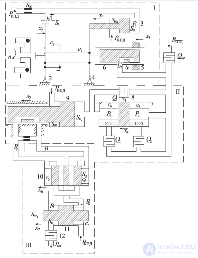
Fig. 3.3. Hydraulic diagram of the speed governor
a
=
Kc12
(1−c1)d32( PКПД − P10 (−Sk +b1′x20)− P10 Sж)
−
2S 2
P
− P
P
11
п1
КПД
10
10
− Kb1′d2 P10 ,
Sп1d1d4
here x2 is the displacement of the valve shutter; PКПД is the constant pressure; P1 is the working pressure; Sж is the jet cross-sectional area; Sk is the initial cross-section of the regulated valve; b1′ is the width of the regulated valve's orifice; Sп1, Sш1 are the areas of the hydraulic cylinder's piston and rod; d1–d4 are the lever arms; K is a coefficient characterizing the properties of the working fluid; c1, c2 are the spring stiffnesses; KГ is the coefficient of the centrifugal sensor.
The derivation of the analytical values of the coefficients b1, a11 is
given in [25].
The isodrome regulator controls the position of the metering needle (MN). The flow cross-sectional area of the MN determines the amount of fuel supplied to the combustion chamber. The hydraulic diagram of the isodrome regulator is shown in Fig. 3.3 (loop II) and consists of a control slot 6 on the physical-speed sensor's rod, an isodrome piston 7, a throttling pack 8, and a metering needle 9.
The mathematical model of the isodrome regulator has the form
dx4
= b u +a
x ,
dt
1
11
4
(3.17)
dx5
= b u + a
21
x ,
dt
2
5
where x4
is the displacement of the isodrome;
x5
is the displacement of the MN;
u =
d3
x − x
( x
–
displacement
of the sensor's hydraulic cylinder; x –
d4
1
3
1
3
displacement of the mode-setting lever);
b =
Kb2′
P30
;
1
S1
b =
Kb2′
P30
;
2
Sп2
c +c
Qдр
Kb′u
0
Q
a = −
3
4
+
2
+
iz
;
11
S 2
P
−
Р
Р
P
− Р
1
КПД
30
30
30
40
146
c +c
Qдр
Kb′u
0
a
21
= −
3
4
+
2
;
S S
п2
P
−
Р
1
КПД
30
P30 , P40 are the pressures in the working cavities of the system; c3, c4 are the spring stiffnesses;
S1 is the area of the isodrome;
Sп2 , Sш2 are the areas of the piston and rod of the metering needle; b2′ is the width of the regulated slot's orifice;
Qдр are the discharge coefficients;
K is a coefficient characterizing the properties of the working fluid. The derivation of the analytical values of the coefficients b1, b2 , a11, a21
is given in [25].
The fuel pressure drop across the flow cross-section of the MN profile is maintained by the constant-pressure-drop valve (CPDV), which controls the position of the swash plate of the pumping unit.
The hydraulic diagram of the CPDV is shown in Fig. 3.3 (loop III) and consists of a spool valve 10, a hydraulic cylinder 11, and a throttling pack 12.
The mathematical model of the CPDV has the form
dx7
= b u +b u
ext
+ a
x ,
(3.18)
dt
1 1 2
11
7
where x7 is the displacement of the CPDV's hydraulic-cylinder piston;
uext is the external influence, uext = f (n,αsp) ( n is the rotational speed of the engine's HPC rotor; αsp is the swash-plate tilt angle (the dependence uext = f (n,αsp) is shown in Fig. 3.3));
u1 = x6 is the displacement of the CPDV's spool valve;
a
= −Kc
(S
+b′
x
)(K P
(S
+b′
x
) +Q P′− P
) /
2(S
− S
)2
×
11
7
0
60
70
0
60
др
70
п3
ш3
×(K P
(S
+b′
x
)( P′− P + P′′
− P
) +Q P′
− P P′′− P
+
70
0
60
70
80
др
70
80
+(−Kc
)(S
+b′
x
)(K P
(S
+b′
x
) +Q P′− P
) / 2(S
− S
)2 ×
7
0
60
70
0
60
др
70
п3
ш3
×(K P70 (S0 +b′
x60
)( P′− P70 +
P′′− P80 ) +Qдр P′− P70 P′′− P80 ;
147
b = −K(S
+b′
x
)(K P (S
+b′
x
) +Q P′− P ) / 2(S
− S
)2 ×
1
0
60
70
0
60
др
70
п3
ш3
;
×(K P (S
+b′
x
)( P′
− P + P′′− P ) +Q P′
− P P′′− P
70
0
60
70
80
др
70
80
b2 = −Kb′(S0 +b′
x60
)( P′− P70 + P′′− P80 ) P′′− P80 (K P70 (S0 +b′
x60
) +
2
+Qдр P′− P70 ) / (Sп3
− Sш3 )
(K P70 (S0
+b′
x60
)( P′− P70 + P′′− P80 )×
′ ′
− S
)
2
×(1+Q )] + Kb P
− P / (S
п3
ш3
.
др
70
P′ = P50 ,x60 > 0;
P60 ,x60 < 0
P′′ = P60 ,x60 > 0;
P50 ,x60 < 0
P50, P60 – pressures upstream and downstream of the metering needle;
P70, P80 – operating pressures;
Sп3, Sш3 – piston and rod areas of the KPP (constant pressure-drop valve) hydraulic cylinder; c5, c6, c7 – spring stiffnesses;
b′ – width of the opening in the spool;
S0 – area of the initial opening in the spool; Qдр – throttle discharge coefficient;
K – coefficient characterizing the properties of the working fluid. The derivation of the analytical values of the coefficients b1, b2, a11 is given
in [25].
Thus, the formalization of the HMA carried out using the example of the engine shaft speed governor (as the most complex subsystem of the pump-governor) showed that the element-wise models of the individual HMA subsystems are typical elements, such as a first-order lag element and a real integrating element with a summed input having nonlinear parameters.
The formalization of the remaining subsystems of the pump-governor is given in [25].
An analysis of the features of the mathematical models of the main components of the pump-governor showed that the element-wise models of the individual subsystems of the pump-governor can be represented by the following types of elements:
148
1. First-order lag element:
dx1
= b u + a
x .
(3.19)
dt
1
11
1
This type of mathematical model corresponds to:
the constant pressure-drop valve (KPP),
the actuating element of the engine-inlet temperature sensor, and the physical speed sensor.
2. Ideal integrating element:
dx1
= bu.
(3.20)
dt
This type of mathematical model corresponds to: the starting automatic
device and the mechanism for maintaining minimum fuel flow
3. Real integrating element:
dx1
= b u
+ a
x
,
dt
1
11
1
(3.21)
dx2
= a
21
x .
dt
1
This type of mathematical model corresponds to: the IGV control mechanism on the RA, the fuel supply control unit operated by signals from the OA, and the HPC bleed valve (ZPV KVD) control mechanism on the RA.
4. Real integrating element with a summed input:
dx1
= b u + a
x ,
dt
2
11
1
(3.22)
dx2
= b u + a
21
x .
dt
2
1
This is the mathematical description of an isodromic (rate) governor.
5. Third-order element: series connection of a first-order lag element and a real integrating element:
dx1
= b u
+ a x ,
dt
1
11
1
dx2
= a
x +a
22
x ,
(3.23)
dt
21
1
2
dx3
= a
x .
dt
32
2
This is the mathematical description of the IGV unit operated by signals from the OA. The classification performed defines the range of models inherent
to the object of the class under study and makes it possible to select an identification method.

Comments