
Lecture
Identification theory is a branch of applied mathematics and systems analysis that deals with building mathematical models of dynamic systems based on data about the behavior of those systems. The main goal of identification is to create models that can accurately describe the behavior of a system, even if its internal structure is partially or completely unknown.
Key aspects of identification theory include:
System modeling: creating a mathematical model that describes the dynamics of the system. Models can be linear or nonlinear, deterministic or stochastic.
Data collection: identifying a system requires data on the system's input and output signals (e.g., data on the system's response to external influences).
Parameter estimation: the main task is to find the model's parameters, such as coefficients, that best describe the system. Optimization methods are used to minimize the difference between observed data and model results.
Identification methods:
Identifiability: this is a property of a system that indicates whether it is possible to uniquely determine the model's parameters based on the available data.
Model validation: after identification, a check is performed on how well the model corresponds to the actual behavior of the system, using test data or other approaches such as cross-validation.
Examples of applications of identification theory include automatic control, diagnostics and forecasting of technical systems, biological systems, financial models, and other complex dynamic processes.
At present, problems related to creating mathematical models of objects in technological processes, economics, and living nature form one of the main directions of science and technology — modeling. This is because mathematical models of objects are widely used both in creating control systems for these objects and in their operation.
This textbook considers only models of technical objects and systems. Objects and systems are a collection of material bodies in continuous interaction with each other and with the environment. Building a mathematical model of an object can be done using several methods: analytical, experimental, and experimental-analytical [1–3].
The analytical method involves obtaining a mathematical description of an object based on the laws of physics, mechanics, chemistry, and so on. Such an approach yields a positive result if the object under consideration is sufficiently simple in structure and well studied. If, however, the object is insufficiently studied or so complex that describing it analytically with a mathematical model is practically impossible, experimental methods are used, the essence of which comes down to the statistical processing of process data. In the experimental-analytical method, an a priori model obtained analytically is refined in corresponding experiments.
The interaction of an object with the environment can be represented as shown in the figure (Fig. 1.1).
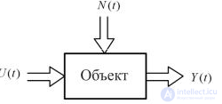
Fig. 1.1. Block diagram of the controlled object
These influences are called external. Among external influences, the following are distinguished: U(t) — input influences, N(t) — disturbing influences.
The second group of environmental influences changes the object's state variables indirectly, usually non-additively. These influences lead to a change in the object's (system's) operator A, by which is meant the law governing the transformation of input influences into the object's output variables. Such influences are called operator influences.
The behavior of the object is described by the vector Y(t).
The scheme of interaction with the environment can be represented in more detail (Fig. 1.2).
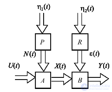
Fig. 1.2. Block diagram of the controlled object's model
The following notation is used in the diagram:
• U(t), Y(t) — observed input and output signals. They
can be deterministic or random, and can be a mixture (usually additive) of deterministic and random components. Input signals can be specially applied to the system for identification purposes (active experiment), or they can exist in the system as control or disturbing influences (passive experiment);
•X(t) — unobserved signals, estimated indirectly from the signal Y(t) obtained as a result of transformation in the object by operator B;
•η1(t), η2(t) — unobserved disturbances, which are typically
random processes of the white noise type, in some cases containing matching deterministic components;
• N(t), ε(t) — usually unobserved, typically time-correlated
random signals, in some cases containing deterministic components;
• A, B, P, R — operators, whose form is in some cases unknown, and in others known but with unknown parameters.
According to the block diagram of the object's model given above (see Fig. 1.1), the main identification tasks are the following:
1. The task of finding the characteristics (parameters) of the object.
Given the known observed variables U(t), Y(t), it is required to determine the operators (or the parameters of the operators) A, B. Often, along with determining the parameters A, B, it is also necessary to establish the parameters of the operators P, R, which transform the unobserved white noise η1(t), η2(t) into the unobserved signals N(t), ε(t).
2. The task of estimating state variables.
The state of the object is characterized by the vector of state variables X(t), a vector that uniquely determines all its characteristics. Given the known observed signals U(t), Y(t), and with the operators A, B, P, R known along with their parameters, it is required to determine (estimate) the unobserved signal X(t). Sometimes the task of jointly estimating parameters and state arises.
3. The task of generating random signals with specified characteristics, or determining the characteristics of random signals.
Given the observed variables N(t), ε(t), it is required to determine the operator (or the parameters of the operator) P, R.
The identification task includes the following stages:
•formulating requirements for observational data: how to carry out the collection of experimental data, and how to use this data collected under real experimental conditions;
•defining the class of objects — the set of candidate models from which the best model will subsequently be selected;
•forming a so-called loss or risk function (optimality criterion) that characterizes the adequacy of the object and the model being tuned, and on that basis formulating a criterion for the quality of identification;
•choosing a way to assess the degree to which the model under study corresponds to the experimental data;
•defining a model verification procedure: carrying out a check
and confirmation of the model's adequacy, i.e., determining to what extent the model actually "explains" the behavior of the system under study.
The following factors play a significant role in building mathematical models.
1. Before starting the experiment, it is necessary to determine the conditions under which data collection will be carried out, and to resolve questions about the further specific use of that data. These tasks are addressed at the experiment-planning stage by choosing the number of experimental trials and the conditions for conducting them, necessary and sufficient for solving the stated problem with the required accuracy. This stage does not directly belong
to identification, but precedes it.
2. In a constructive sense, identification is the determination, from input and output influences, of a model from a certain class of models to which the real system under study is equivalent.
Accordingly, it is necessary to define the class of models from which the most suitable one will be selected. At this stage, it is necessary to choose the general structure of the model and the class of equations intended to describe the observed process. This stage is sometimes called identification in the broad sense (or structural identification) and often turns out to be the decisive factor. Successfully solving the structural identification problem requires the use of a priori information about the physical, chemical, or other phenomena occurring in the process, knowledge of the formal analytical properties of models, engineering skills, and intuition. To this day, no general formal approaches to solving the structural identification problem exist, and the structural identification stage often comes down to a heuristic specification of the model structure based on a priori information about the object.
3. The closeness of the resulting model to the real system under study is fairly relative, since the operators of the object and of the model may be described in different languages, and may have different structures or numbers of inputs, and therefore the concept of adequacy can be formulated in different ways. Since it is difficult or often impossible to directly assess the closeness of the operators of the object and the model, what is most often assessed is the closeness of the output values of the object and the model, or the mathematical expectation of parameter estimation errors. For this purpose, the concept of a loss or risk function is introduced, which is subsequently subject to minimization. Then, in order to select the "best" model from a given class based on this loss function, a certain criterion is formed, and the identification problem thereafter becomes a problem of optimizing the chosen criterion.
4. After determining the structure of the model and the class of equations, it is necessary to establish the numerical values of the parameters — the coefficients of differential, difference, integral equations, or other mathematical constructs of the linear or nonlinear model of the object and (or) the states included in the equations of the mathematical model. Thus, the task to be solved is the estimation of parameters and (or) states based on available experimental data, i.e., based on the values of measured variables. This task is called the parametric identification problem (or identification in the narrow sense). When estimating parameters, one has to solve the problem of minimizing certain functional dependencies on measured quantities (usually on the difference between the output signals of the model and the object) and on unmeasured quantities — parameters and states. To solve this problem, it is necessary to develop an identification algorithm that, based on the input and output quantities available for observation, would determine the parameters of the model being tuned that minimize the error of the model description in accordance with the chosen quality functional.
5. The transition from the model-building stage to its subsequent use requires an assessment of the quality of the resulting model, i.e., verification of the model's adequacy to the object. Because absolute equivalence between the model and the object is fundamentally unattainable, the main condition for confirming the adequacy of the resulting model is the possibility of using it to solve the problem for which the model was built. Adequacy therefore implies that the model reproduces, with the necessary completeness, all properties of the object that are significant for the purposes of the given study. The degree of adequacy between the model and the object is usually assessed by comparing their output signals when the same input influences are applied to the object and to its model. This comparison is preferably carried out using new information, different from the data that was used in the process of identifying the object.
In most real situations, the interaction of an object with the environment corresponds to the following standard scheme (Fig. 1.3):
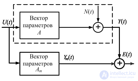
Fig. 1.3. Typical observation scheme for object identification
The following notation is used in the diagram: U(t) — vector of input influences;
Y(t) — vector of the object's output influences; Ym(t) — vector of the model's output influences;
N(t) — vector of uncontrolled random influences;
E(t) — vector of the difference (residual) between the outputs of the object and the model;
A — vector of the object's parameters; Am — vector of the model's parameters.
The identification experiment, according to the observation block diagram, consists of the following.
An external influence is applied to the inputs of the object and the model. Under real conditions of the object's interaction with the environment, the observation signals of the object are distorted by random disturbances determined by the specific nature of the object's own functioning, by errors of measurement methods and instruments, and by uncontrolled influences of the external environment. When using such an observation scheme, it is assumed that the generalized noise vector N(t) includes all external disturbances, deviations of measured values from true influences, and other factors. Typically, as a result of the experiment, observations of the input and output are obtained, i.e., realizations of the random functions U(t) and Y(t).
The law governing the object's functioning can be represented as follows:
Y(t) = F0(U(t), N(t), A). (1.1)
According to relation (1.1), the object's output value depends on the external influence U(t), the disturbance N(t), and the unknown parameter vector A, whose values are not directly observable.
Based on information about the object, a model is formed, understood as some operator F that transforms the observed input influence U(t) into its response Y(t):
Ym(t) = F(U(t), Am). (1.2)
Model (1.2) is described by equations similar to the object's equations (1.1) and containing information about the measured input and output values, with the assumption that noise does not change the form of the model. The coefficients of these equations are the model's parameters. The model's output value depends on the parameters Am, which
are calculated based on an algorithm that processes the vector of all observations. To find the parameter vector Am, it is necessary to determine the optimal way, in the sense of similarity to the object, to adjust the model. With this approach, the identification task consists of constructing a model operator F from a certain class of operators (the structural identification problem) and determining, from the observations U(t) and Y(t), the parameter vector Am (parametric identification), such that the model's output signal is as close as possible to the object's output signal.
Based on comparing the object's output signal Y(t) = F0(U(t), N(t), A), distorted by the disturbance N(t), with the model's output signal Ym(t) = F(U(t), Am), the residual is calculated — the difference between the output values of the object and the model:
E(t) = Y(t) − Ym(t). (1.3)
To assess how well the model corresponds to the object, a loss function (residual function) F(Y(t), Ym(t), A) is introduced, which depends on the outputs of the object and the model and on the model's parameters.
Based on the residual function, an identification criterion is formulated:
J(Y, Ym, A) = J{F(Y, Ym, A)}. (1.4)
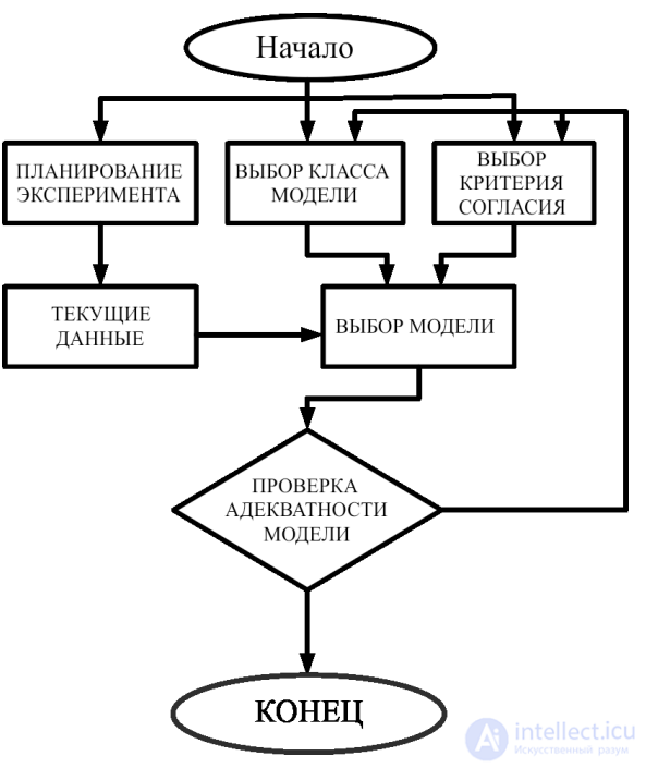
Fig. 1.4. General scheme of model identification
The identification quality criterion, which characterizes the adequacy of the model to the real object, represents the average loss. The smaller the average loss, the higher the quality of identification.
Minimizing the identification functional, which corresponds to improving the quality of identification, is carried out by appropriately choosing the model's structure and changing the values of its parameters. This adjustment procedure is implemented by the identification algorithm.
There are various ways of estimating parameters, which differ from one another in the optimality criterion used and in the available a priori information. To a certain extent, the choice of optimality criterion is subjective, and the estimation procedure depends significantly on the criterion adopted.
The general identification scheme is shown in Fig. 1.4.

Comments