
Lecture
Methods for estimating the parameters of object models can generally be divided into two classes depending on how the estimation procedure is implemented. The first type includes approaches based on the use of explicit mathematical expressions, while the second type includes estimation procedures implemented using an adjustable (tunable) model.
When implementing estimation methods of the first type (Fig. 1.6), the mathematical model is given in the form of explicit mathematical relations containing a set of numerical values A to be determined.
Identification experiments are conducted on the object to collect arrays of input U(t) and output Y(t) data. The results are then processed. Based on the experimental data obtained, a model is constructed that ensures the minimum value of the functional J(Y, Ym, Am). The optimal estimation procedures
for the parameters A in this case reduce to solving the following equation:
дJ
= 0.
(1.13)
дA
m
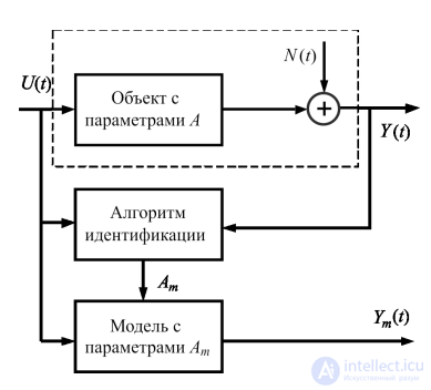
Fig. 1.6. Explicit scheme for implementing the identification algorithm
In this case, parameter estimation is carried out using retrospective identification algorithms, in which the solution is obtained by processing the entire data array through a finite number of elementary operations and cannot be obtained as a result of intermediate computations. From an engineering standpoint, such an estimation procedure belongs to identification methods performed outside the control loop and does not allow incoming observations to be processed sequentially, in normal operating mode.
A block diagram of the estimation procedure based on an adjustable model [12–14] is shown in Fig. 1.7.
When implementing estimation methods of the second type (see Fig. 1.7), the principle of adjusting the model to the object based on closeness of behavior is used. In this case, the model of the object under study, represented by parameters Am, is changed so that
the model's characteristics become close to the characteristics of the system under study. The optimal procedures for estimating the parameters Am in this case reduce to solving the following equation:
дJ → 0. (1.14)
дAm
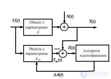
Fig. 1.7. Scheme for implementing the identification algorithm with an adjustable model
The residual E(t) is fed to the input of the identification algorithm block, which changes the parameters of the adjustable model Am based on
the solution of equation (1.14). In principle, the solution is obtained as the result of an infinite number of such operations, with each intermediate result representing an approximate solution.
This type of implementation belongs to closed-loop identification methods and allows real-time identification to be carried out while the object is operating normally.
It should be noted [15–17] that with the advent of digital computing devices it has become more convenient to implement the required functions (criterion computation, automatic tuning, etc.) algorithmically, which leads to a blurring of the clear boundaries between different identification approaches. The main feature indicating the use of identification methods with an adjustable model should be considered the presence of feedback.
Among the possible identification algorithms, the recursive least squares (LS) method and the stochastic approximation method (SAM) have become widely used. The least squares method corresponds to minimization of the quadratic criterion (1.10). The SAM is characterized by simplicity and versatility and makes it possible not to be limited to quadratic identification criteria, but to form a variety of both linear and nonlinear identification algorithms.
The features of each of the identification algorithm implementation schemes are given in Table 1.1.
Table 1.1
1.4.2. Classification of control object models
There is a wide variety of types and classes of models. None of the classification methods gives a complete picture or reflects all the properties of the models used, since each characterizes only individual features of a model.
Let us consider the main types of models, divided according to the main systemic features [6, 9].
1. Physical (real-world/scale) and mathematical (symbolic). Physical models are those in which the properties of the real
object are represented by the characteristics of a real object of the same or similar nature.
Mathematical models are those in which mathematical constructs are used to describe the characteristics of the object. In what follows, we will consider only mathematical models.
2. One-dimensional and multidimensional.
Objects having one input and one output are called one-dimensional, while multidimensional (multiply-connected) objects have several inputs and several outputs.
3. Static or dynamic.
An object is called dynamic if its output response depends not only on the input action at the current moment in time but also on previous values of the input. This means that the object possesses inertia (memory). Mathematical models of dynamic objects describe its behavior over time.
An object is called static if its response to an input action does not depend on its history, on the system's past behavior, or on previous values of the input. Static systems have an instantaneous response to an input action, and their models describe processes that do not change over time, i.e., the behavior of the object in steady-state modes.
4. Linear or nonlinear.
An object is called linear if the superposition principle holds for it, i.e., the object's response to a linear combination (superposition) of two input actions equals the same combination of the object's responses to each of the actions individually:
f (α1u1(t) +α2u2 (t)) = α1 f (u1(t)) +α2 f (u2 (t)) ,
(1.15)
where u1(t), u2(t) are input actions; α1, α2 are arbitrary coeffi-
cients.
Otherwise the object is considered nonlinear. 5. Stationary or non-stationary.
An object is called stationary if its response to identical input actions does not depend on the time at which these actions are applied, i.e., the parameters of such an object do not depend on time.
Otherwise, the object is said to be non-stationary.
6. Discrete or continuous.
An object is called continuous if the state of its input and output actions changes or is measured continuously over a certain time interval.
An object is called discrete if the state of its outputs and inputs is defined only at discrete moments in time. To de-
25
scribe discrete systems, lattice (grid) functions are used, which are analogs of continuous functions, and difference equations, which are analogs of differential equations.
7. Deterministic or stochastic.
An object is called deterministic if its output action is uniquely determined by the structure of the object and the input actions and does not depend on uncontrolled random factors. In real conditions, observed output signals change not only under the influence of observed inputs but also due to numerous unobserved random disturbances. If these disturbances are small or absent, the system can be considered deterministic.
A system in which random disturbances have a significant effect on the output variables is called stochastic. A stochastic (probabilistic) model reflects the influence of random factors, so between the input and output variables there is not a unique functional dependence but a probabilistic one. Usually, the state variables of a stochastic object are estimated in terms of mathematical expectation, while the input actions are described by probability distribution laws.
8. Lumped and distributed.
An object is called an object with lumped parameters if its input and output quantities depend only on time (only on one variable). Models of objects with lumped parameters contain one or more time derivatives of the state variables and are ordinary differential equations. The mathematical model of transient processes in an object, along with the differential equation, also contains additional uniqueness conditions — initial conditions.
An object is called an object with distributed parameters if the output quantity depends on several variables — on time and on spatial coordinates. Such a situation usually occurs when the characteristic of the object under study, for example, temperature, substance concentration, and others, is distributed within a certain volume. In this case the mathematical model of the object contains partial derivatives and describes both the dynamics of the process in time and the distribution of the characteristic in space. The mathematical model of processes in a distributed object includes a differ-
26
ential equation in partial derivatives, initial conditions, and boundary conditions. An example of such a model can be the wave equation, a diffusion model, or a heat conduction model:
дQ(x, t)
= a
д2Q(x, t)
+ f (x, t, u(x, t)),
(1.16)
дt
дx2
where Q(x, t) is the state function of a one-dimensional object with distributed
parameters x [x0, x1], and a, f are given coefficient and func-
tion, respectively.
9. "Input–output" characteristics and description in state space.
"Input–output" type characteristics are certain operators that relate the behavior of the object's output quantity to the input, for example, the transfer, transient, and impulse-response (weighting) functions.
State-space models describe the dynamic behavior of a system with n coordinates, called state coordinates. Such coordinates, for example, are the values of a function and its n − 1 derivatives at an arbitrary point in time. They form an n-dimensional vector that fully determines the state of the system at any moment in time in the n-dimensional state space or phase space.
The coordinates of the state vector, unlike the vectors of input and output quantities, are generally abstract mathematical characteristics whose physical nature is not essential. The coordinates of the state vector, as well as the structure and values of the coefficients of the state equations, depend on the choice of basis
in the phase space.
10. Structured and aggregated.
A structured model is a representation of the mathematical model of the entire system as a whole as a set of relatively simpler models of individual elements and blocks of the object, interconnected by links. It characterizes both the physical and technical aspects of constructing a control system and allows the study of processes occurring both in the system as a whole and in its individual elements. Thus, a structured model of a control system represents a set
of a number of interrelated mathematical models of individual links. In such a model, by successively eliminating from consideration all internal variables that are input or output signals of internal links, one can find a differential equation describing the relationship between the input and output quantities of the system, which is essentially an aggregated model.
An aggregated model describes the functional relationships between input and output quantities without taking into account the internal structure and interconnections in the system.
11. Parametric and non-parametric.
Parametric models are described by explicitly given analytical dependencies containing parameters subject to identification. These dependencies represent finite-dimensional parametric models, for example, differential equations of a certain order, or state-space models. The parameters are the numerical values of the quantities determining the model's output (for example, the values of the coefficients of ordinary differential equations, initial conditions, or the coefficients of transfer functions). Parametric identification methods are used to determine the unknown coefficients of the object equation or transfer function.
Non-parametric models reduce to a description of transformations of signals from the input space into elements of the output space. In this case the object model is defined by an operator that transforms functions of input signals into functions of output quantities. Non-parametric models include weighting functions, transfer functions (if the number of coefficients is not specified in advance), correlation functions, spectral densities, and Volterra series. For example, for a model in the form of a weighting function, the relationship between input and output signals for linear objects is given by means of the convolution integral (Duhamel integral):
∞∞
y(t) = ∫w(t)u(t −τ)dτ = ∫u(t)w(t −τ)dτ,
(1.17)
0
0
where w(t) is the impulse transient (weighting) function of the object, which is a non-parametric model of a linear dynamic object.
Non-parametric identification methods are used to determine the time or frequency characteristics of objects. From the characteristics obtained, the transfer function or the equations of the object can then be determined. Parametric models can lead
28
to large errors if the order of the model does not correspond to the order of the object. The advantage of non-parametric models is
that they do not require explicit knowledge of the order of the object. However,
in this case the description is, in essence, infinite-dimensional.
The main classes of models have the following mathematical description.
1. Static models.
The static characteristic of an object is the relationship between the input and output signals in steady-state mode. Analytically, in the general case, the equation of a static object model has the form of a nonlinear function of many variables:
y = f (u).
(1.18)
In many practical cases, the general nonlinear function (1.18) can be parameterized by some vector A, and then this dependence takes the form
y = f (u, A)
(1.19)
and the identification problem reduces to determining the unknown parameters A.
A special case of parametric models [3, 13] are models that are linear with respect to the parameters being estimated:
y = a0 +a1u1 +K+ anun.
(1.20)
The model of a static linear multidimensional object with n inputs and m outputs is a system of linear algebraic equations:
y = a + a u + a u
2
+K+ a
u
n
,
1
10
11 1
12
1n
y2 = a20 + a21u1 +a22u2 +K+ a2nun ,
(1.21)
M
y
m
= a
m0
+ a
u + a
m2
u
2
+K+ a u
n
,
m1
1
mn
where aij are the unknown parameters of the model to be determined.
In vector-matrix form, system (1.21) takes the form
Y = A0 + AU ,
(1.22)
29
where U and Y are the vectors of input and output actions; A0 and A are, respec-
tively, the vector and matrix of model coefficients to be identified.
The mathematical description (1.20) is called one-dimensional linear regression, and (1.21)–(1.22) — multidimensional linear regression. In practice, most problems can be reduced to linear regression, so the identification of linear regression parameters is an important task and will be considered below.
2. Linear dynamic continuous parametric models. Linear dynamic continuous models in control theory
can be given in the following forms:
• Ordinary differential equations of order n:
a
d n y(t)
+ a
d n−1 y(t)
+K+ a
n
y(t) =
dtn
dtn−1
0
1
(1.23)
d m x(t)
d m−1x(t)
= b
+b
+K+b x(t),
dtm
dtm−1
0
1
m
where ai, bj (i =1,n, j =1,m) are the model parameters to be identi-
fied. For most real physically realizable control systems, m ≤ n.
• Transfer functions.
If zero initial conditions are set for the differential equation (1.23), then, applying the Laplace transform, the transfer function of the linear object is obtained in the following form:
y( p)
b pm +b pm−1
+K+b
W ( p) =
=
0
1
m
,
(1.24)
x( p)
a pn + a pn−1
+K+ a
0
1
n
where p is a complex variable — the parameter of the Laplace transform.
• State-space equations.
Dynamic processes, along with the n-th order differential equation (1.24), can also be described by a system of n ordinary first-order differential equations:
dyi (t)
n
m
= ∑aij y j +∑biju j , i =
.
(1.25)
1,n
dt
j=1
j=1
Introducing a state vector of the system into the description, we represent the state-space model in the following matrix form:
dX (t) = AX (t) + BU (t),
(1.26)
dt
Y (t) = CX (t) + DU (t),
where X(t) is the vector of internal (dynamic) variables;
U(t) is the
vector of input variables; Y(t) is the vector of output variables; A is the matrix of system coefficients; B is the system's input matrix; C is the system's output matrix; D is the system's feedforward (bypass) matrix.
Taking into account the influence of the external environment, in the presence of an additive input
disturbance N(t) and measurement errors ε(t),
the basic formu-
lation of the model has the form
dX (t) = AX (t) + BU (t) + KN(t),
(1.27)
dt
Y (t) = CX (t) + DU (t) +ε(t),
where, in addition to the notations discussed earlier, there are also N(t), the vector of random disturbances; ε(t), the vector of measurement noise; and K, the matrix describing the disturbance transmission channel.
The disturbances N(t) and ε(t) are usually assumed to be Gaussian random processes in the form of white noise.
The model under consideration (1.27) can be represented by a block diagram in state space (Fig. 1.8).
Fig. 1.8. Block diagram of a linear dynamic system in state space, taking into account the influence of the external environment
31
3. Linear dynamic discrete parametric models. Linear dynamic discrete models can take
the following forms [2, 6, 17]:
• Ordinary difference equations.
A universal characteristic for discrete models is the n-th order difference equation, which uses the concept of a difference as an analog of the concept of a derivative for continuous models:
an y(k) +an−1 y(k −1) +K+ a0 y(k −n) =
(1.28)
= bmu(k) +bm−1u(k −
1) +K+b0u(k −m),
where y(k), u(k) are the values of the output and input quantities at the k-th moment in time.
• Discrete transfer functions.
Applying the time-shift operator z, defined by the relation y(k +i) = zi y(k), to the finite-difference equation (1.28), we obtain the operator form of the discrete model:
y(z)
b +b
z−1
+K+b z−m
W (z) =
=
m
m−1
0
.
(1.29)
x(z)
a
+K+ a z−n
+ a
n−1
z−1
n
n
• State-space equations.
Using discrete state variables to describe
the dynamics of a discrete
object, forming an
n-dimensional state
x (k)
1
vector
X (k) =
x2
(k)
a description of the object in state
M
,
xn
(k)
space is obtained in the following vector-matrix form:
X (k +1) = AX (k) + BU (k),
(1.30)
Y (k) = CX (k) + DU (k).
A structural representation of model (1.30) is shown in Fig. 1.9.
32
U (k)
X (k +1)
X (k)
Y (k)
B
z−1
C
A
D
Fig. 1.9. Block diagram of a discrete model
in state space
4. Nonlinear dynamic models.
The class of nonlinear dynamic systems is significantly broader compared to linear systems, since these systems exhibit a wide variety of phenomena and processes not characteristic of linear systems. As a result, the mathematical apparatus of linear systems theory becomes inapplicable for describing such systems, so when solving the problem of obtaining mathematical models of nonlinear systems, the following two main approaches are used [15, 18]. One approach consists of obtaining an approximate mathematical description of a linearized model (essentially determining a model equivalent to the original nonlinear model) using linearization methods: harmonic, statistical, or the small-increment method. This approach is most applicable for objects having smooth characteristics and for processes occurring with small deviations and perturbations relative to nominal operating modes.
In the second approach, the mathematical model is considered to be essentially nonlinear. In this case, the most common types of models are the following:
• Nonlinear differential equations.
For a continuous one-dimensional control object, the relationship between the input and output signals is written in general form as the implicit expression
dy
, K,
d n y
, u,
du
, K,
d mu
= 0,
(1.31)
F y,
dtn
dt
dt
dtm
33
where F is a certain nonlinear operator that needs to be identified. If possible, the nonlinear model (1.31) is parameterized based on structuring F with the introduction of some parameter vector A:
F y, dy
, K,
d n y, u, du, K,
d mu, A
= 0.
(1.32)
dt
dtn
dt
dtm
In this case, the identification problem reduces to determining the operator F and estimating its parameter vector A.
For a nonlinear discrete object, analogous nonlinear difference equations are constructed.
• Hammerstein models.
Such models of nonlinear systems with memory (inertial objects) are constructed on the assumption that the nonlinearity and inertia of the object can be separated, i.e., it can be represented as a series combination of two elements: a nonlinear memoryless (static) element and a linear dynamic element. "Input–output" models for such objects in the one-dimensional stationary case can have two variants of description:
∞
y(t) = ∫w(τ)F(u(t −τ))dτ
(1.33)
0
or
∞
(1.34)
y(t) = F ∫w(τ)u(t −τ)dτ ,
0
where w(τ) is the impulse transient function of the linear element;
F(u) is the
static characteristic of the nonlinear element.
A structural representation of the object model for each of the description variants is shown in Figs. 1.10–1.11.
Fig. 1.10. Block diagram of the Hammerstein model (1.33)
34
Fig. 1.11. Block diagram of the Hammerstein model (1.34)
• Volterra series expansion.
In this method of description, the relationship between the input u(t)
and the output y(t)
is represented by the series [1, 3]
t
t t
y(t) = ∫w1
(τ)u(t −τ)dτ+ ∫∫w2
(τ1,τ2 )u(t −τ1)u(t −τ2 )dτ1τ2 +... , (1.35)
0
0 0
where w1(τ), w2(τ1,τ2), w3(τ1,τ2,τ3)K are the generalized weighting functions (ker-
nels) of order i. Such a series (1.35) is called the Volterra series. The Volterra series expansion is a direct generaliza-
tion of the linear model in the form of a convolution integral to nonlinear objects. The identification problem in this case consists of determining the generalized weighting functions w1(τ), w2(τ1,τ2), w3(τ1,τ2,τ3)K. For a non-
stationary object, the kernels will depend on t.
• Description in state space.
In the general case, the state equations for finite-dimensional continuous systems are written in the following form:
dx(t)
= f (x(t), u(t), t),
dt
y(t) = g(x(t), u(t), t),
(1.36)
x(t0 ) = x0.
In the general case, in equations (1.36) the nonlinear functions f and g are to be determined. If they can be parameterized by some parameter vector A, the description of the system takes the form
dx(t)
= f (x(t), u(t), A, t),
dt
y(t) = g(x(t), u(t), A, t),
(1.37)
x(t0 ) = x0.
35
The state-space equations for discrete nonlinear objects, when the nonlinear functions are parameterized by A, take the form
x(k +1) = f (x(k), u(k), A),
y(k) = g(x(k), u(k), A),
(1.38)
x(k0 ) = x0.
State-space representation is particularly convenient for multidimensional objects. For non-stationary objects, it is necessary to introduce a time dependence for the vector A.
1.4.4. Controllability, observability, and identifiability of systems
Important concepts for the study of systems, including for identification, are the concepts of controllability, observability, and identifiability of systems [3, 7, 8].
Let us consider each of these concepts in more detail.
A system is controllable if it can be transferred from any initial state X(t0) to any other desired
state X(tk) over a finite time interval τ (τ = tk − t0) by specifying (varying) the input action U(t).
The concept of controllability can be illustrated by the following example (Fig. 1.12).
Fig. 1.12. Block diagram of an uncontrollable system
It is obvious that this system is uncontrollable, since the control action u(t) does not affect all the state
variables (the state variable x4(t) cannot be controlled).
36
A system is observable if all state variables can be determined, directly or indirectly, from the system's output vector.
Whereas controllability requires that every state of the system be sensitive to the input action, observability requires that every state of the system affect the measured output vector.
A distinction should be made between the concepts of "measurability" and "observability." To measure a variable directly using measuring devices means to record the value of the variable at the current moment in time directly using measuring instruments. An observable variable is one that is either measured directly or computed on the basis of measured variables.
The concept of observability can be illustrated by the following example (Fig. 1.13).
Fig. 1.13. Block diagram of an unobservable system
It is obvious that this system is unobservable, since not all state variables X(t) can be reconstructed from the measured output vector Y(t) (ME — measuring element). Thus, the dynamic variable x5(t) is unobservable.
An automatic control system (ACS) is identifiable if the model's parameters can be determined from the vector of state variables.
The controllability, observability, and identifiability of a system are determined by the following criteria.
37
Let the description of the ACS be represented in terms of state space as
dX (t)
= AX (t) + BU (t)
,
(1.39)
dt
Y (t) = CX (t) + DU (t)
where X(t) is the vector of internal (dynamic) variables;
U(t) is the
vector of input variables; Y(t) is the vector of output variables; A is the matrix of system coefficients; B is the system's input matrix; C is the system's output matrix; D is the system's feedforward (bypass) matrix.
The system will be controllable only if the controllability matrix has rank n, where n is the order of the system (i.e., the order of the state vector X(t)):
M y =[BM ABM A2 BMKAn−1B], (1.40) rank(M y ) = n.
The system will be observable only if the observability matrix has rank n, where n is the order of the system (i.e., the order of the state vector X(t))
T
T T
T 2
T
T
n−1
C
T
Mн = C
M A C
M (A )
C
MK(A )
,
(1.41)
rank(Mн) = n.
The system will be identifiable if the identifiability matrix has rank n, where n is the order of the system (i.e., the order of the state vector X(t)).
Mи = V (0)M AV (0)M (A)2V (0)MK(A)n−1V (0) , (1.42) rank(Mи) = n.
1.4.5. Identification of a linear regression model
The most widely used method of parameter estimation, serving as the basic approach to parametric identification, is the least squares method, which, under the assumption of linearity and time-discreteness of the object, leads to the simplest and most universal solutions. The problem is as follows: given
38
the available sample data of observations of the input and output signals, it is required to estimate the values of the parameters that ensure the minimum value of the residual functional between the model and actual data:
J = ET IE → min.
(1.43)
The residual function
E =Y −Ym
(1.44)
represents the difference between the output of the object under study, Y, and the response computed from the mathematical model of the object, Ym. The re-
sidual is made up of inaccuracies in the model structure, measurement errors, and unaccounted-for interactions between the environment and the object. However, regardless of the origin of the resulting errors, the least squares method minimizes the sum of the squared residual values.
In principle, the least squares method does not require any a priori information about the disturbance. But in order for the resulting estimates to have desirable properties, we will assume that the disturbance is a random process of the white-noise type.
An important property of least-squares estimates is the existence of only one local minimum, which coincides with the global minimum. Therefore the estimate Am is unique. Its value is determined
from the extremum condition of the functional (1.43):
дJ = 0. (1.45)
дAm
Estimation of a linear system by the least squares method is called linear regression analysis, owing to the linear operator of the model.
Let us turn to the fundamentals of linear regression analysis for estimating the parameters of one-dimensional and multidimensional linear static systems [7, 14, 19].
Consider the linear static system shown in Fig. 1.14, having n inputs U and one output y.
This system can be described by the following linear equation:
y = a0 +a1u1 +K+ anun.
(1.46)
39
Fig. 1.14. One-dimensional system diagram
u1
Using a series of measurements of the quantities U = u2 and y over a cer-
Mun
tain time interval t [t0, tk], a measurement matrix of the quantities U and Y can be formed as follows:
u (1)
u
(1)
L
u
n
(1)
U =
1
2
,
u1(2)
u2 (2)
L
un (2)
M
(k) u2 (k) L
u1
un (k)
y(1)
Y =
y(2)
,
M
y(k)
where ui(j) is the value of the i-th input variable,
measured at the moment
in time t j = t0 + j∆t; ∆t
is the sampling interval, ∆t =
tk −t0
.
k
Equation (1.46) can be rewritten in vector-matrix form:
Ym =UAm ,
(1.47)
where U is a unit column, introduced for the identification of the parame-
1
u (1)
u
(1)
K u
n
(1)
1
2
ter
a ,
U = 1
u1(2)
u2 (2)
K un (2)
;
0
M
M
M
M
M
1 u1(k) u2 (k)
K un (k)
a0
Am is the matrix of model coefficients, Am = a1 .
Man
The estimation error, or residual function, has the form
y(1)
ym (1)
E =Y −Y
= y(2)
− ym (2) .
(1.48)
m
M
M
y(k)
ym (k)
Then the optimality criterion is determined by the least squares method:
J = ET E.
(1.49)
Thus, the best (in the least-squares sense) estimate of the matrix Am is determined as the solution of the following equation:
дJ
= 0.
(1.50)
дA
m
After substituting (1.48) into (1.49), equation (1.49) takes the form
дJ
д{ET E}
д{(Y −Y )T (Y −Y )}
=
=
m
m
=
дA
дA
дA
m
m
m
(1.51)
д{(Y −UA )T
(Y −UA )}
=
m
m
= 0.
дAm
Equation (1.50) represents the differentiation of the scalar
quantity ET E with respect to the matrix A,
using matrix algebra, we trans-
m
form expression (1.50):
41
дJ
д{(Y −UA )T (Y −UA )}
дtr{(Y −UA )(Y −UA )T }
=
m
m
=
m
m
=
дA
дA
дA
m
m
m
= дtr(YYT +UAm (UAm )T −Y (UAm )T −UAmY )T =
дAm
= дtr(YYT +UAm AmTU T −YAmTU T −UAmY )T =
дAm
дβααT γ
T
T
=
(β γ
+ γβ)α
∂α
=
дβαT γ
= γβ
=
дα
дβαγ
T
T
дα
=β γ
= 0 +(U T (U T )T +U TU )A
−U TY −(U )T (YT )T =
m
= (U TU +U TU )A −U TY −U TY =
m
= 2U TUA −2U TY = 0,
m
where tr is the trace of the matrix.
Equation (1.50), after transformation, has the form
U TUA −U TY = 0.
(1.52)
m
Thus, the best estimate of the parameter matrix Am in the least-squares sense satisfies the equation
A =[U TU ]−1U TY = 0.
(1.53)
m
This expression forms the basis for identification based on linear regression and the least-squares method.
For the constructed model to be adequate to the object, the number of measurements k must satisfy the following condition:
k ≥ n +1.
(1.54)
One-dimensional linear regression analysis can also be applied to nonlinear systems. Let us illustrate this with the following example.
Suppose the system is described by a quadratic equation
42
y = a0 + a1x + a2 x2.
It is easy to see that equation (1.54) is applicable to equation (1.45) provided that u1 = x, u2 = x2. Then the matrix U is defined as
x(1)
x
2
(1)
1
1 x(2)
x2
(2)
U =
.
M
M
M
x(k)
x
2
1
(k)
a0
The parameter vector A = a1 is estimated using
a2
formula (1.52).
Consider the linear static system shown in Fig. 1.15, having n inputs U and m outputs Y.
Fig. 1.15. Diagram of a multivariable system
The process occurring in multivariable systems has n inputs and m outputs and, by analogy with the one-dimensional process, can be described by the following system of equations:
n
y1 = a10 +∑a1iui
i=1
M
(1.55)
n
ym = am0 +∑amiui . i=1
43
u1
Using a series of measurements of the quantities U = u2 and Y
Mun
y1
= y2
over the
M
ym
course of a certain time interval t [t0 , tk ], we can form the matrix of measurements of the quantities U and Y as follows:
1
U = u1(1)M
un (k)
y1(1)
Y = Mym(1)
1 u1(2)
un (k)
y1(2)
ym(2)
L
1
L
u
(k)
1
L
un (k) .
Lym(k)
M
Lym(k)
Equation (1.55) can be rewritten in matrix form:
Ym = AmU.
(1.56)
Let us compute the optimal estimate of the matrix A in a manner analogous to that used for one-dimensional systems:
дJ
д(ET E)
д(Y −Y )T (Y −Y )
=
=
M
M
=
дA
дA
дA
m
m
m
= дtr[(Y − AmU )(Y − AmU )T ] =
дAm
= дtr(YYT + AmU (AU )T −Y (AmU )T − AmUYT ) =
дAm
= дtr(YYT + AmUU T AmT −YU T AmT − AmUYT ) =
дAm
44
дαβαдα T = α(β+βT )
=
дβαT
=β
=
дα
дβαγ
T
T
дα
=β γ
=0 + Am (UU T +(UU T )T ) −YU T −(I )T (UYT )T =
=Am (UU T +UU T ) −YU T −YU T =
= 2AmUU T −2UX T = 0.
Thus, the best estimate of the parameter matrix Am in the least-squares sense satisfies the equation
A =YU T (UU T )−1.
(1.57)
m
The requirements on the number of measurements are such that, for the model to be adequate, it is necessary that:
l ≥ (n +1) m.
(1.58)
The methods discussed above for estimating one-dimensional and multivariable linear models are implemented using an explicit identification scheme, whose advantages and disadvantages were discussed above.
In practice it is more advisable to apply iterative methods, i.e., schemes with an adjustable model.
Linear regression analysis can be implemented in a closed identification scheme (a scheme with an adjustable model).
Iterative identification methods use methods of successively refining the coefficient matrix.
The formula for iterative regression analysis has the form
A (k +1) = A (k) +[Y (k +1) − A (k)U (k)][P(k +1)U (k)]T , (1.59)
m
m
m
where Am (k +1), Am (k) are the estimated coefficient matrix at the previous and current observation instants, respectively; Y (k +1) is the output vector measured at the current (k +1) observation instant; U (k) is the input vector measured at the previous k-th observation instant; P(k +1) is an auxiliary matrix determined by the formula
45
P(k +1) = P(k) − P(k) U (k)×
×[1+U T (k)P(k)U (k)]−1U T (k)P(k). (1.60)
Iterative computations are carried out until the refinement of the coefficients of the matrix Am (k +1) reaches the specified accuracy:
Am (k +1) − Am (k)
≤ ε.
(1.61)
The initial values of the matrices Am (0), P(0) can be chosen arbitrarily, for example, as follows:
A(0)
= I,
P(0)
=
1
I,
(1.62)
ε
where I is the identity matrix; ε is the specified estimation accuracy.
1.4.6. Identification of dynamic systems
The identification of dynamic systems is generally based on describing these systems in terms of a transfer function [7, 13, 21].
Suppose a dynamic system is described by a transfer function of the following form:
W(p)=
b pm +b pm−1
+...+b
p +b
0
1
m+1
m
.
(1.63)
a pn + a pn−1
+...+ a
p + a
0
1
n−1
n
Based on the transfer function (1.63) we obtain a system of first-order differential equations consisting of n equations
dx
= AX(t)+ BU(t),
(1.64)
dt
Y(t)= CX(t),
where Y(t) is the vector of output variables; U(t) is the vector of input
variables; X(t) is the state vector (internal dynamic variables).
From the differential equations we move to difference equations
46
V(k +1)= Ф(Т )V(k),
0Y(k)= СV(k),
U
where V is the generalized vector, V = ; Ф(bi , ai , T0 )
X
(1.65)
is the transition matrix, whose parameters bi , ai are to be estimated.
In accordance with (1.57) and (1.65) the transition matrix Ф is determined
as
Ф(Т0)=V T (k +1)V T (k)V(k)V T (k) −1,
(1.66)
where
V(k)=
v1(1)
v1(2)
L v1(l −1)
M
M
,
vn(1) vn
(2)
L vn(l −1)
v
(2)
v
(3)
L
v (l)
V(k +1)=
1M
1
1M
.
vn
(2) vn
(3)
L vn(l)
The number of measurements l is determined by formula (1.58).
From the obtained transition matrix, the coefficient matrix can be computed:
∞ (AT )i
AT
Ф(T ) − I
Ф(T0 ) = ∑
0
≈ I +
0
A ≈
0
.
(1.67)
i!
1!
T
i=0
0
Example.
Suppose the control object is given by the block diagram (Fig. 1.16):
u(t)
x2 (t)
x1(t)
K1
T
K2
−
y(t)
1T
Fig. 1.16. Block diagram of the automatic control system
47
It is necessary to determine the system parameters K1, K2, T. Let us define the system state vector:
r V = x1 .
x2
The dynamics of the processes are described by a system of differential equations:
drdt = 0,
dx1
= K
2
x ,
dt
2
dx2
=
K1
r −
K1
x −
1
x ,
dt
T
T
1
T 2
y = x1.
The main matrices of the model:
0
0
0
A =
0
0
K
2
,C =[0 1 0].
K
K
1
1
−
1
−
T
T
T
The coefficient matrix
A
has dimension n×n = 3×3, so
for reliable identification results (1.58) the number of observations l must be at least 10.
As a result of a series of experiments, the state vector is determined:
r(1)
K
r(10)
V = x
(1)
K
x
(10)
,
1
1
(1)
K
x2
x2
(10)
and the matrices V (k), V (k +1), respectively, have the form
48
r(1)
K
r(9)
(1)
V (k) = x1
K
x1(9) ,
(1)
K
x2
x2 (9)
r(2)
K r(10)
V (k +1) =
(2)
x1
K x1(10) .
(2)
x2
K x2 (10)
Then the transition matrix can be determined:
Ф(T0 ) =V (k +1) V T (k) V (k) V T (k) −1,
and, based on the transition matrix, the coefficient matrix as well:
A ≈ Ф(T0 ) − I. T0
Knowing the numerical values and structure of the coefficient matrix A, one can determine the system parameters K1, K2, T.
1.4.7. Identification of nonlinear systems
The fairly well-developed theory of identification of nonlinear systems offers a large number of different methods for studying them. However, none of the methods is universal, and each is characterized by its own domain of application. The most widely used methods are the following [3, 7, 21]:
1. Direct search method.
2. Approximation of the nonlinearity.
3. Hammerstein model.
4. Wiener method.
5. Two-stage procedure. Let us consider each of the methods.
1. Direct search method.
The nonlinear function f(x) is converted into a linear function fL(x). Then any method for identifying linear systems is applied.
Suppose the object model has the form
y = α
0
xβ1 xβ2
,
(1.68)
1
2
49
where x1, x2 are input variables; y is the output variable; α0, β1, β2 are
the estimated model parameters.
It is easy to see that taking the logarithm of the nonlinear equation
(1.68) reduces the system to a linear form:
z = a0 +a1r1 + a2r2 ,
(1.69)
where z is the output variable of the linear model,
z = lny ;
r1, r2 are the input variables of the linear model, r1 = lnx1, r2 = lnx2 ; a0, a1, a2 are the parameters of the linear system, a0 = lnα, a1 =β1, a2 =β2.
The parameters of the linear model are estimated using the explicit methods of one-dimensional linear regression (1.52) or the iterative method (adjustable-model scheme) (1.59).
2. Approximation of nonlinearities.
In accordance with the Weierstrass theorem, any continuous nonlinear function can be represented as a polynomial
y = a
+ a x + a
2
x2
+b х
2
+b х2
+K .
(1.70)
0
1
1
1
1
2
2
Polynomial (1.70) is easily reduced to a linear regression, whose estimation algorithm was discussed above.
Approximation using a polynomial is convenient when the values of the nonlinear function are obtained experimentally.
3. Hammerstein model.
In accordance with the Hammerstein model, the nonlinear system is reduced to the form shown in Fig. 1.17.
Fig. 1.17. Block diagram of the Hammerstein model
The identification algorithm depends on the prior information about the form of the nonlinearity F(u(t)).
If the functional dependence F(u(t)) is known, then, by introducing the variable z(t) = F(u(t)), identification reduces to determining the parameters of the linear part of the Hammerstein model:
y(t) =W ( p)z(t).
(1.71)
If the functional dependence F(u(t)) is not known, a table of this nonlinear dependence is constructed, from which an approximating polynomial of the nonlinearity P(u(t)) is calculated using any interpolation formula. Knowing the parameters of the approximating polynomial, the variable z(t) = P(u(t)) is determined, and the identification problem again reduces to determining the parameters of the linear part of the Hammerstein
model (1.71).
4. Wiener method.
The Wiener method is one of the most accurate methods for identifying nonlinear systems.
The essence of the method consists in sequentially expanding the input signal, first in terms of Laguerre coefficients:
т
x(t) ≈ ∑ci xi ,
(1.72)
i=1
where ci are the Laguerre coefficients; xi
are the discrete values of the input
signal.
The Laguerre coefficients are calculated by the formula
ci =
xi
,
(1.73)
(n +1)2 L
(x )2
n+1
i
where Ln+1(xi) is the value of the Laguerre polynomial computed for the discrete signal value xi.
The recurrence formula for computing the Laguerre polynomial has the form
(n +1)Ln+1(x) = (2n +1− x)Ln (x) −nLn−1(x).
(1.74)
The Laguerre coefficients are represented in the form of a Hermite function:
c
= (−1)
i
e
i 2 d(e−x )
(1.75)
.
i
dxi
The Hermite functions and the output signals of the object under study are compared by a special cross-correlator, which determines the reliability of the identification performed.
This approach has the following advantages:
51
•Stationary white Gaussian noise is the most general test signal for a stationary nonlinear system.
•Any nonlinear system has an equivalent in the form of a certain linear system (a Laguerre chain) with many outputs, followed by a memoryless system (a Hermite function).
However, the Wiener approach has limited practical application. This is due to the following reasons:
•The requirement that the input be white Gaussian noise is too strict. It is much more convenient to have a method capable of processing signal realizations during normal operation.
•The number of coefficients required to describe even a simple nonlinear system is very large.
•Wiener's theory does not allow obtaining a description of nonlinear systems that admits a clear physical interpretation.
5. Two-stage procedure for identifying nonlinear systems. The procedure for estimating the parameters of a nonlinear object is
carried out in two stages.
1) The nonlinear characteristic is divided into sections within which the nonlinear function can be represented, with sufficient accuracy, by a linear function (Fig. 1.18).
Fig. 1.18. Linearization of a nonlinear dependence
The sections [xi, xi+1] are called linearization sections; the beginning of the sections xi is called the linearization point. At each
продолжение следует...
Часть 1 1.4. Parametric Identification
Часть 2 - 1.4. Parametric Identification

Comments