Statistical training

The main concepts in this chapter, as well as in chapter 18, are data and hypotheses. But in this chapter, data is considered as evidence, i.e. fleshing out some or all of the random variables describing the problem domain, and the hypotheses are probabilistic theories of how the problem domain functions, including logical theories as a particular case.

Consider a very simple example. Our favorite lollipops "Surprise" are available in two varieties: cherry (sweet) and lemon (sour). The candy manufacturer has a special sense of humor, so it wraps each candy in the same opaque paper, regardless of the variety. Candies are sold in very large packages (also outwardly indistinguishable), which are known to be of five types: h1: 100% cherry candies h2: 75% cherry + 25% lemon candies h3: 50% cherry + 50% lemon h4 candy: 25% cherry + 75% lemon candy h5: 100% lemon candy

After receiving a new packet of candies, the candy lover tries to guess what type it belongs to, and indicates the type of packet to the random variable I (short for hypothesis, a hypothesis), which has possible values ​​from h1 to h5. Of course, the value of the variable I cannot be determined by direct observation. As sweets are deployed and inspected, data about them is recorded. where each data item , is a random variable with possible values ​​of cherry (cherry candy) and lime (lemon candy). The main task facing the agent is that he must predict which variety the next candy belongs to. Despite the apparent simplicity, the statement of this problem allows you to familiarize yourself with many important topics. In fact, the agent must logically derive a theory about the world in which he exists, although very simple.

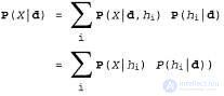
In Bayesian training, the probability of each hypothesis is simply calculated from the data obtained and predictions are made on this basis. This means that predictions are made using all the hypotheses, weighted by their probabilities, and not using only the “best” hypothesis. Thus, learning is reduced to probabilistic inference. Assume that the variable D represents all the data, with the observed value of d; in this case, the probability of each hypothesis can be determined using Bayes' rule:

(20.1)

Now suppose that it is necessary to make a prediction regarding an unknown number of X. In this case, the following equation applies:

(20.2)

where it is assumed that each hypothesis determines the probability distribution over X. This equation shows that the predictions are the weighted averages of the predictions of the individual hypotheses. The hypotheses themselves are essentially “intermediaries” between factual data and predictions. The main quantitative indicators in the Bayesian approach are the distribution of a priori probabilities of the hypothesis, , and the likelihood of data according to each hypothesis,

With reference to the example with candy, suppose that the manufacturer announced the presence of a distribution of a priori probabilities over the values , which is defined by the vector <0.1,0.2,0.4,0.2,0.1>. The likelihood of the data is calculated according to the assumption that the observations are characterized by the iid property, i.e. are independent and equally distributed (iid - independently and identically distributed), therefore the following equation is observed:

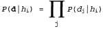(20.3)

For example, suppose a package is actually a package of this type, which consists of some lemon candies and all the first 10 sweets are lemon candies; in this case, the value equally

, because in a package of type h3, half of the candies are lemon candies2. In fig. 20.1, and it is shown how the posterior probabilities of five hypotheses change as we observe the sequence of 10 lemon drops. Note that the probability curves begin with their a priori values, so the h3 hypothesis is initially the most likely option and remains so after the deployment of 1 candy with lemon candy. After deploying 2 candies with lemon candies, the h4 hypothesis becomes the most likely, and after detecting 3 or more lemon candies, the h5 hypothesis becomes the most likely (a hateful package consisting of only sour lemon candies). After the discovery of 10 lemon candy in a row, we are almost certain of our ill-fated fate. In fig. 20.1.6 shows the predicted probability that the next candy will be lemon, according to equation 20.2. As expected, it monotonously increases to 1.

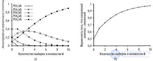
Fig. 20.1. Change in probabilities depending on the amount of data: a posteriori probabilities obtained using equation 20.1. The number of observations N increases from 1 to 10, and in each observation is detected lemon candy (a); Bayesian predictions derived from equation 20.2 (b)

This example shows that the true hypothesis will ultimately dominate the Bayesian prediction. This is a characteristic feature of Bayesian learning. For any given distribution of a priori probabilities, which does not exclude the true hypothesis from the very beginning, the posterior probability of any false hypothesis ultimately completely disappears simply because the probability of the indefinitely long formation of "uncharacteristic" data is vanishingly small (compare this with discussing ASD learning in chapter 18). More importantly, Bayesian prediction is optimal, regardless of whether a large or small data set is used. If there is a distribution of a priori probabilities of the hypothesis, all other predictions will be correct less often.

But for the best Bayesian training, of course, you have to pay. In real learning tasks, the hypothesis space is usually very large or infinite, as shown in Chapter 18. In some cases, the operation of calculating the sum in equation 20.2 (or, in the continuous case, the operation of integration) can be performed successfully, but in most cases you have to resort to approximate or simplified methods.

One of the most widely used approximate approaches (among those that are commonly used in scientific research) is to make predictions based on the single most probable hypothesis, i.e. that hypothesis which maximizes value . This hypothesis is often called the maximal a posteriori hypothesis, or abbreviated MAP (Maximum A Posteriori; pronounced mi-ey-pi). Predictions made on the basis of the MAP hypothesis are approximately Bayesian to the extent that . In this example, with candy after finding three lemon drops in a row, therefore an agent studying using the MAP hypothesis then predicts that the fourth candy is a lemon candy, with a probability of 1. 0, which is a much more radical prediction than Bayesian prediction of probability 0.8, given in fig. 20.1.

As additional data becomes available, predictions using the MAP hypothesis and Bayes predictions come together, since the emergence of hypotheses that compete with the MAP hypothesis is becoming less and less likely. Although this is not shown in this example, the search for MAP hypotheses is often much easier compared to Bayesian training, since it requires solving an optimization problem, and not a large sum calculation (or integration) problem. Examples confirming this remark will be given later in this chapter.

The distribution of a priori probabilities of the hypothesis plays an important role both in Bayesian learning and in learning using the MAP hypotheses. . As was shown in Chapter 18, if the hypothesis space is too expressive, in the sense that it contains many hypotheses that are in good agreement with the data set, then an overly careful fit can occur. On the other hand, Bayesian teaching methods and teaching methods based on MAR-hypotheses do not impose an arbitrary limit on the number of hypotheses to be considered, but allow the use of a priori probability distribution to impose a penalty for complexity. As a rule, more complex hypotheses have a lower prior probability, partly because there are usually more complex hypotheses than simple ones. On the other hand, more complex hypotheses have a greater ability to fit in with the data (in extreme cases, a search table may be able to accurately reproduce the data with a probability of 1). Therefore, a compromise between the complexity of the hypothesis and the degree of its agreement with the data is embodied in the distribution of a priori probabilities of the hypothesis.

The effect of such a compromise can be observed most clearly in the case of using logical hypotheses, when the variable I contains only deterministic hypotheses. In this case, the value equals 1 if hypothesized speaks with the data, and 0 - otherwise. Considering equation 20.1, we can determine that in such conditions is the simplest logical theory consistent with the data. Therefore, learning with the maximum a posteriori hypothesis is a natural embodiment of the principle of Occam's razor.

Another way to analyze the trade-off between complexity and the degree of consistency is that you can investigate equation 20.1 by taking its logarithm. Applying value to maximize expression is equivalent to minimizing the following expression:

Using the relationship between content and probability, which was described in Chapter 18, we can determine that the term determines the number of bits required to set the hypothesis . In addition, the term represents the additional number of bits required to specify the data, if the hypothesis is given (to verify this, it is sufficient to note that if the hypothesis accurately predicts the data, as in the case of the hypothesis and a whole row of candies with lemon drops, not a single bit is required because ). Thus, learning with the help of the MAP hypothesis is equivalent to choosing a hypothesis that provides maximum data compression. The same problem can be solved more directly using the learning method based on the minimum description length, or abbreviated as MDL (Minimum Description

Length), in which, instead of manipulating probabilities, attempts are made to minimize the size of the hypothesis and the encoded representation of the data.

The final simplification can be achieved by adopting the assumption of a uniform distribution of a priori probabilities over the space of hypotheses. In this case, training using the MAP hypothesis is reduced to the choice of hypothesis which maximizes value . Such a hypothesis is called the maximum likelihood hypothesis (Maximum Likelihood - ML) and is abbreviated as . Training on the basis of the maximum likelihood hypothesis is very widely used in statistics, because in this scientific field many researchers do not trust the distribution of a priori probabilities of a hypothesis, considering that they are subjective. This is an acceptable approach applied in those circumstances when there is no reason to prioritize one hypothesis over another, for example, in those conditions when all hypotheses are equally complex. This training method becomes a good approximation of Bayesian education and training using the MAP hypothesis when the data set is large, since the data corrects the distribution of a priori probabilities for the hypotheses, but is associated with certain problems (as shown below) when using small data sets .