Lecture
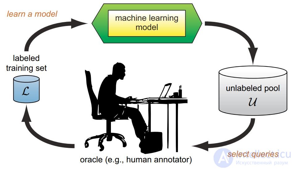
Active learning is distinguished by the fact that the learning algorithm has the ability to independently assign the next situation under study, in which the correct answer will be known.
Active learning is the organization and conduct of the educational process, which is aimed at the full activation of the educational and cognitive activity of students through a wide, preferably complex, use of both pedagogical (didactic) and organizational and managerial tools.
In classical pedagogy, the following didactic prerequisites stand out for the natural intellect.
Content
1 Tasks of active learning
Setting the task of active learning
Active Learning Applications
Active learning strategies
2 Active Learning Strategies
Selecting objects from a selection
Synthesis of objects (planning experiments)
Assessing the quality of active learning
3 Active learning with learning activities
Compromise to learn how to use active learning
Exponential gradient
Active reinforcement training
Task: learning the predictive model a: X → Y according to the sample (xi, yi), when obtaining answers yi is expensive.

Task: learning the predictive model a: X → Y according to the sample (xi, yi), when obtaining answers yi is expensive.
Login: initial tagged sample 
Output: Model A and Marked Sample 
train model a on the initial sample 
until
unallocated objects remain select unallocated object xi;
learn for him yi;
to train model a with one more example (xi, yi);
endpock
The purpose of active learning :
achieve the best quality model a,
using as few additional examples as possible k
Examples of active learning applications
- collection of assessment data for information retrieval, analysis of texts, signals, speech, images, video;
- planning of experiments in the natural sciences (for example, combinatorial chemistry);
- optimization of difficult computable functions (an example is a search in the space of hyperparameters);
- price and assortment management in retail chains;
- selection of goods for marketing campaign.
Pool-based sampling: which next xi to choose from 
Synthesis of objects (query synthesis): at each step, construct the optimal object xi;
Selective sampling: for each xi coming, decide whether to recognize yi
The quality functional of the model a (x, θ) with the parameter θ: 
where L is the loss function, Ci is the cost of information yi for cost-sensitive methods (cost-sensitive)
The idea is to choose xi with the greatest uncertainty a (xi).
The task of multi-class classification: 
where pk (x), k = 1 ... | Y | P (y | x), y ∈ Y, ranked by decrease.
The principle of least confidence (least condence): 
The principle of the smallest indenting margin (margin sampling): 
The principle of maximum entropy (maximum entropy): 
In the case of two classes, these three principles are equivalent.
In the case of many classes, differences appear.
Example. Three classes, p1 + p2 + p3 = 1.
The lines shown are the levels of the three criteria for selecting an object xi

a) min p1
b) min (p1 - p2)
v) 
Example 1. Synthetic data: ℓ = 30, ℓ + k = 400;
(a) two Gaussian classes;
(b) logistic regression for 30 random objects;
(c) logistic regression on the 30 sites selected
through active learning.

Training on biased non-random sampling requires less data to build an algorithm of comparable quality.
Example 2. One-dimensional task with threshold classifier:

Let us estimate the number of steps for determining θ with an accuracy of 1 / k.
Naive strategy: choose  the number of steps is O (k).
Binary search: choose xi closest to the middle of the gap between the classes 
number of steps O (log k)
Idea: choose xi with the most inconsistency of model committee decisions

The principle of maximum entropy: choose xi, on which at (xi) is the most different:

The principle of maximum average KL-divergence: choose xi, on which Pt (y | xi) are the most different:

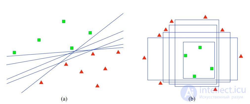
The idea: to choose xi, narrowing as many solutions as possible.
Example. Spaces of admissible solutions for linear and threshold classifiers of cicatories (two-dimensional case):

Boosting and bagging find finite subsets of solutions.
Therefore, disagreement sampling in the committee is an approximation of the principle of reducing the solution space.
Idea: choose xi, which in the stochastic gradient method would lead to the greatest change in the model.
Parametric model of multi-class classification:

For each u ∈ Xk and y ∈ Y, we estimate the length of the gradient steps in the parameter space θ when the model is additionally trained on (u, y);
let ∇θL (θ; u, y) be the gradient vector of the loss function.
The principle of maximum expected gradient length:
xi = arg max
u∈Xk
X
y∈Y
P (y | u, θ)
∇θL (θ; u, y)
Idea: choose xi
which after training will give the most
confident classification of unpartitioned sample X
k
.
For each u ∈ X
k and y ∈ Y will teach the classification model,
adding to tagged training set X
ℓ example (u, y):
auy (x) = arg max
z∈Y
Puy (z | x).
The principle of maximum confidence on unallocated data:
xi = arg max
u∈Xk
X
y∈Y
P (y | u)
X
ℓ + k
j = ℓ + 1
Puy
auy (xj) | xj
.
The principle of minimum entropy of unpartitioned data:
xi = arg max
u∈Xk
X
y∈Y
P (y | u)
X
ℓ + k
j = ℓ + 1
X
z∈Y
Puy (z | xj) log Puy (z | xj
Idea: choose x, which, after the additional training of the model a (x, θ)
will give the smallest estimate of variance σ
2
a
(x).
The regression task, least squares method:
S
2
(θ) = 1
ℓ
X
ℓ
i = 1
a (xi
, θ) - yi
2
→ min
θ
.
From the theory of optimal experiment planning
(OED, optimal experiment design):
x = arg min
x∈X
σ
2
a
(x), σ2
a
(x) ≈ S
2
∂a (x)
∂θ t
∂S
2
∂θ2
−1
∂a (x)
∂θ
.
In particular, for linear regression
σ
2
a
(x) ≈ S
2
x
t
(F
t
F)
−1
x,
where F is the matrix of object attributes.
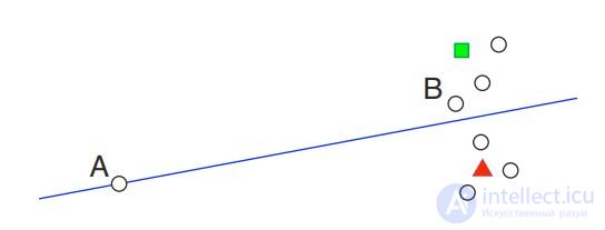
The idea: to reduce the weight of non-representative objects.
Example. Object A is more marginal, but less representative than B.

Any criterion for sampling objects that looks like

can be updated by local density estimation:

sim (x, xj) is an estimate of the proximity of x and xj (the closer, the greater).
Learning curve (learning curve) dependence of the classification accuracy on a test on the number of learning objects.

Learning curves for text classification: baseball vs. hockey. Curve graphics accuracy versus the number of documents requested for two strategy samples: uncertainty sampling (active learning) and random sampling (passive learning). We see that the active approach to learning is higher here, because its learning curve dominates the random sampling curve.
Disadvantages of active learning strategies:
there are untested areas of space X,
as a result, the quality of training decreases,
increases learning time.
Ideas for learning activities:
take a random object with probability ε
adapt parameter ε depending on success
learning activities
use reinforcement training (ontextual MAB)
Djallel Bouneouf et al. Contextual bandit for ative learning: ative Thompsonsampling. 2014
Djallel Bouneouf. Exponentiated Gradient Exploration for Active Learning. 2016
Algorithm wrapping over any active learning strategy
Entry: initial tagged sample X
ℓ = (xi
, yi)
ℓ
i = 1;
Output: Model A and Marked Sample (xi
, yi)
ℓ + k
i = ℓ + 1;
train model a on the initial sample (xi
, yi)
ℓ
i = 1;
while there are unmarked objects
choose unallocated xi randomly with probability ε,
either xi = arg max
x
φ (x) with probability 1 - ε;
learn yi for object xi
;
to train model a with one more example (xi
, yi);
Problem:
how to select the probability ε of research activities?
how to adapt it (reduce) over time?
ε1,. . . , εK is a grid of parameter values ε;
p1,. . . , pK probability use the values of ε1,. . . , εK;
β, τ, κ method parameters.
EG-a algorithm idea
tive: similar to the AdaBoost algorithm,
exponentially increase pk if successful εk:
exponential update of wk scales by value
criteria φ (xi) on the selected object xi
:
wk: = wk exp τ
pk
(φ (xi) + β)
;
probability renormalization:
pk: = (1 - κ) P
wk
j wj
+ κ
one
K
.
Djallel Bouneouf. Exponentiated Gradient Exploration for Active Learning. 2016
EG-active algorithm
Login: X
ℓ = (xi
, yi)
ℓ
i = 1, parameters ε1,. . . , εK, β, τ, κ;
Output: Model A and Marked Sample (xi
, yi)
ℓ + k
i = ℓ + 1;
initialization: pk: = 1
K
, wk: = 1;
train model a on the initial sample (xi
, yi)
ℓ
i = 1;
while there are unmarked objects
choose k from a discrete distribution (p1, ..., pK);
choose unallocated xi randomly with probability εk,
either xi = arg max
x
φ (x) with probability 1 - εk;
learn yi for object xi
;
to train model a with one more example (xi
, yi);
wk: = wk exp
τ
pk
(φ (xi) + β)
;
pk: = (1 - κ) Pwk
j wj
+ κ
one
K
Disadvantages of active learning strategies:
- there are not surveyed areas of space X,
- as a result, the quality of training decreases,
- increases the time of training.
Ideas for using contextual bandit (ontextual MAB):
- actions (pens) are clusters of objects,
- the context of the cluster is its vector indicative description,
- the premium encourages model change a (x, θ),
- linear model is used to select actions.
Djallel Bouneouf et al. Contextual bandit for active learning: active Thompson sampling. 2014
William R. Thompson. On the other hand, it’s another view. 1933.
C many actions (pens, clusters of objects),
btc ∈ R
n is the feature vector of the cluster c ∈ C at step t,
w ∈ R
n vector coefficients of the linear model.
Game agent and environment (
ontextual bandit with linear payo):
initialization of a priori distribution p1 (w);
for all t = 1,. . . , T
the environment informs the agent btc contexts for all c ∈ C;
the agent samples the vector of the linear model wt ∼ pt (w);
agent chooses action ct = arg max
c∈C
hbtc, wti;
Wednesday generates rt premium
;
the agent adjusts the distribution according to the Bayes formula:
pt + 1 (w) ∝ p (rt
| w) pt (w);
A priori and a posteriori Gaussian distributions.
Game agent and environment (
ontextual bandit with linear payo):
initialization: B = Inchn; w = 0n; f = 0n;
for all t = 1,. . . , T
the environment informs the agent btc contexts for all c ∈ C;
agent sampled linear model vector
wt ∼ N (w, σ2B
−1
);
agent chooses action ct = arg max
c∈C
hbtc, wti;
Wednesday generates rt premium
;
the agent adjusts the distribution according to the Bayes formula:
B: = B + btcb
t
tc; f: = f + btc rt
; w: = b
−1
f;
The recommended value of the constant σ
2 = 0.25.
Agent and environment play (we build active learning)
C: = clustering unpartitioned sample X
k
;
initialization: B = Inchn; w = 0n; f = 0n;
for all t = 1,. . . , T, while unallocated objects remain
calculate btc contexts for all clusters c ∈ C;
Sample the vector of the linear model wt ∼ N (w, σ2B
−1
);
select cluster ct = arg max
c∈C
hbtc, wti;
select random unpartitioned xi from ct cluster
;
learn for him yi
;
to train model a with one more example (xi
, yi);
calculate the premium rt (the formula on the next slide);
adjust the distribution by Bayes formula:
B: = B + btcb
t
tc; f: = f + btc rt
; w: = b
−1
f;
Idea: the premium encourages a model change of a (x, θ).
Ht =
a (xi
θt)
ℓ + k
i = 1 vector of answers on sample X
ℓ ∪ X
k
The premium angle between the vectors Ht and Ht − 1:
rt
: = e
βt
arccos
hHt
, Ht − 1i
kHtk kHt − 1k
,
where the exponential factor compensates for decreasing distances;
β = 0.121 is an empirically selected parameter.
Djallel Bouneouf et al. Contextual bandit for active learning: active Thompson sampling. 2014
btc =
Mdisc, Vdisc, | c |, plbtc, MixRatetcy
Mdisc mean intracluster distance;
Vdisc dispersion of intracluster distances;
| c | the number of objects in the cluster;
plbtc the proportion of marked objects in the cluster;
MixRatetcy is the fraction of objects of class y ∈ Y in the cluster.
Total Features: 4+ |
R (T) = P
T
t = 1
hbtc ∗
t
, wti - hbtc, wti
,
c
∗
t optimal action (R = 0 if all actions are optimal)
Comparison of accumulated losses for different algorithms
A passive learner agent is guided by a constantly defined strategy that determines his behavior, and the active agent must decide for himself what actions to take. We begin with a description of an agent acting through adaptive dynamic programming, and consider what changes need to be made to his project so that he can function with this new degree of freedom.
First of all, the agent will need to determine through training the full model with probabilities of results for all actions, and not just a model for a given strategy. The simple learning mechanism used in the Passive-ADP-Agent algorithm is excellent for this purpose. Then it is necessary to take into account the fact that the agent must make a choice from a variety of actions. The benefits that he will need for training are determined by the optimal strategy; they obey the Bellman equations given in p. 824, which we again give below for convenience.
 (21.4)
Эти уравнения могут быть решены для получения функции полезности U с помощью алгоритмов итерации по значениям или итерации по стратегиям, приведенных в других статьях (гл17). Последняя задача состоит в определении того, что делать на каждом этапе. Получив функцию полезности U, оптимальную для модели, определяемой с помощью обучения, агент может извлечь информацию об оптимальном действии, составляя одношаговый прогноз для максимизации ожидаемой полезности; еще один вариант состоит в том, что если используется итерация по стратегиям, то оптимальная стратегия уже известна, поэтому агент должен просто выполнить действие, рекомендуемое согласно оптимальной стратегии. Но действительно ли он должен выполнять именно это действие?
Активное обучение используется для уменьшения обучающей выборки, когда размеченные данные дороги
Active learning is faster than passive
With a small amount of marked data, it reaches the same quality as passive with full markup
The introduction of learning activities in active learning allows you to explore space X even faster
To this end, in recent years, adaptive strategies or reinforcement training have been applied.
Comments
To leave a comment
Machine learning
Terms: Machine learning