
Lecture
Logarithmic amplitude-phase frequency response (commonly abbreviated LAFChKh in Russian; in English usually called a Bode diagram or Bode plot) — a representation of the frequency response of a linear time-invariant system on a logarithmic scale.
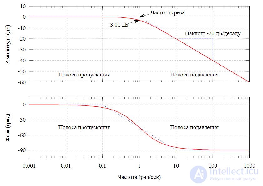
The Bode plot is built as two graphs: the logarithmic amplitude-frequency response and the logarithmic phase-frequency response, which are usually placed one below the other.
LAFR is the dependence of the magnitude of the gain (voltage, current or power) of a device, ( , or for power
  , on frequency, on a logarithmic scale.
The abscissa axis plots frequency on a logarithmic scale, the unit of measurement being a dimensionless quantity:
The ordinate axis plots the amplitude of the output signal in logarithmic dimensionless units:
PFR is the dependence of the phase difference between the output and input signals on frequency, on a semi-logarithmic scale
Nepers and octaves are now obsolete and are practically never used.
The reason for plotting amplitude and phase characteristics on a logarithmic scale is the ability to study the characteristics over a wide range.
The actual LAFR and PFR are rarely used in practice.
For a clearer analysis of the characteristics, their modified versions are used — the asymptotic logarithmic amplitude-frequency response and the asymptotic logarithmic phase-frequency response, in which the curve is replaced by segments of a broken straight line. The word “asymptotic” is usually dropped, but it must always be remembered that the asymptotic responses and the LAFR (PFR) are different characteristics.
Analysis of systems using the asymptotic PFR is quite simple and convenient, and it is therefore widely used in various branches of technology, such as digital signal processing, electrical engineering and control theory.
In Western literature the name Bode diagram or Bode plot is used, after the outstanding engineer Hendrik Wade Bode.
In engineering circles the name is usually shortened to LAR.
In the applied engineering computation packages GNU Octave and MATLAB, the function bode is used to plot the Bode plot.
If the transfer function of a system is rational, then the Bode plot can be approximated by straight lines. This is convenient when drawing the Bode plot by hand, and also when composing the Bode plot of simple systems.
The Bode plot is convenient for the synthesis of control systems, as well as digital and analog filters: in accordance with specified quality criteria, the desired Bode plot is constructed, approximated by straight lines, which is then broken down into the Bode plots of individual elementary blocks, from which the transfer function of the system (controller) or filter is reconstructed.
On the LAFR graph, the abscissa is frequency on a logarithmic scale, and the ordinate axis plots the amplitude of the transfer function in decibels.
Representing the amplitude-frequency response on a logarithmic scale simplifies the construction of the characteristics of complex systems, since it allows the operation of multiplying the amplitude-frequency responses of blocks to be replaced by addition, which follows from the property of the logarithm:  .
.
On the graph of the phase-frequency response, the abscissa is frequency on a logarithmic scale, and the ordinate axis plots the phase shift of the system's output signal relative to the input signal (usually in degrees).
A variant is also possible in which the ordinate axis plots the phase shift on a logarithmic scale; in that case the characteristic is called the PFR.
The amplitude and phase of a system rarely change independently of each other — when the amplitude changes, the phase changes too, and vice versa. For minimum-phase systems, the PFR and LAFR can be uniquely determined from each other using the Hilbert—Warrington transform.
The basic idea is based on the following mathematical rule of adding logarithms. If the transfer function can be represented as a fractional-rational function
 ,
,
then:

After splitting the transfer function into elementary blocks, the Bode plot of each individual block can be constructed, and the resulting Bode plot obtained by simple addition.
When constructing the LAFR, the scale  is usually used for the ordinate axis, that is, an amplitude-frequency response value of 100 becomes 40 decibels on the LAFR scale. If the transfer function has the form:
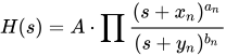
where  — is a complex variable that can be related to frequency using the following formal substitution:
  ,
,  and
and  — are constants, and
  — is the transfer function. Then the LAFR can be constructed using the following rules:
where  (a zero), the slope of the line increases by
  dB per decade. where
  (a pole), the slope of the line decreases by
  dB per decade.
 into the transfer function.
 , and the slope changes at the point
  at once by
  dB per decade.
To correct the LAFR approximated by straight lines, one must:
 dB above the line (
 dB for two complex-conjugate zeros) dB below the line ( dB for two complex-conjugate poles)
To construct the approximated PFR, the transfer function is written in the same form as for the LAFR:
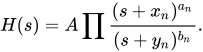
The basic principle for constructing the PFR is to draw separate graphs for each pole or zero, then add them together. The exact curve of the phase-frequency response is given by the equation:
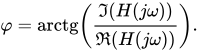
To draw the PFR for each pole or zero, the following rules are used:
 is positive, start the line (with zero slope) at 0 degrees, is negative, start the line (with zero slope) at 180 degrees,
 (
( for a complex-conjugate one) degrees per decade starting at
 (
( for a complex-conjugate one) degrees per decade starting at
  degrees for a simple zero or pole, and by
  degrees for a complex-conjugate zero or pole,
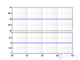
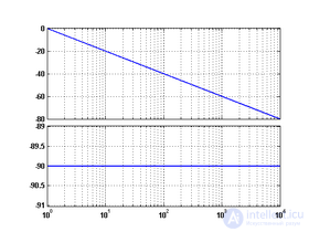
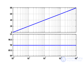
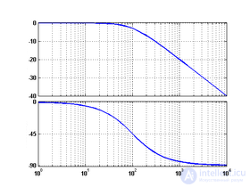
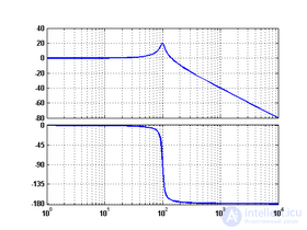
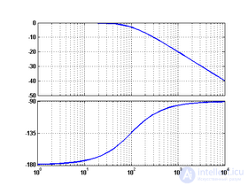
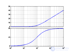
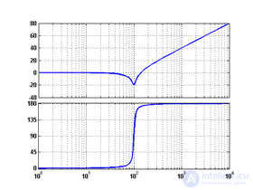
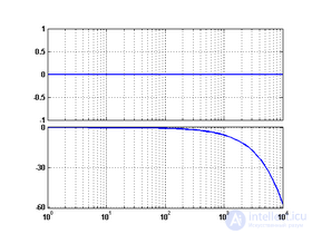
Below is a table listing the transfer functions and Bode plots of some typical elementary blocks. Most linear time-invariant systems can be represented as a combination of such blocks. In the table, — is a complex variable.
| No. | Block | Transfer function | Bode plot | Notes |
|---|---|---|---|---|
| 1 | proportional |  |
 |
 |
| 2 | ideal integrating |
 |
 |
|
| 3 | ideal differentiating |
|
 |
|
| 4 | aperiodic (real integrating) |
 |
 |
 |
| 5 | oscillatory | 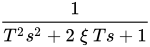 |
 |
 |
| 6 | unstable aperiodic |
 |
 |
non-minimum- phase |
| 7 | differentiating first order (first-order |
 |
 |
|
| 8 | lead second order |
 |
 |
|
| 9 | pure delay |
 |
 |
 |
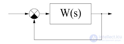
The determination of system stability is based on a model in the form of a block enclosed by negative feedback and the possibility of it entering self-oscillation (the oscillatory stability boundary). The condition for self-oscillation is the presence of positive feedback, in which case the gain in the forward path must be no less than unity. The phase of the output signal (described by the phase-frequency response), through the negative feedback path, is fed back to the input, and the “phase margin” is defined as the additional phase shift that must occur at the output in order to produce positive feedback. The gain in the forward branch is described by the amplitude-frequency response, and the frequency at which the gain is unity is called the “cutoff frequency”; on the LAFR the cutoff frequency is the point where the characteristic crosses the abscissa axis. Graphically, the phase margin is defined as the difference between a phase of π radians (180°) and the phase at the cutoff frequency (the condition for positive feedback to form); the “gain margin” is the distance along the amplitude axis from the cutoff-frequency point to the amplitude at an angle of π radians (the condition for unity gain in the forward branch).
To determine the stability of a closed-loop system, the Bode plot of the open-loop system is constructed (see figure). Next, one must find the cutoff frequency ωc by solving the equation  (here and below
  ; if there are several roots, the largest root must be chosen), and the frequency ω180 — the largest of the frequencies for which
 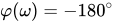 . Then
 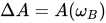 — is the gain margin,
  — is the phase margin. If these margins are negative, the closed-loop system is unstable; if they equal zero, it is at the stability boundary.
This algorithm is applicable only to minimum-phase systems . In other cases, the Nyquist—Mikhailov and Routh—Hurwitz stability criteria can be used to determine stability.

Comments