Elliptic Integral: Essence and Applications

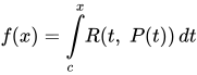
An elliptic integral is a function f over the field of real or complex numbers that can be formally represented in the following form:

,

where R is a rational function of two arguments, P is the square root of a polynomial of degree 3 or 4 with no repeated roots, and c is some constant from the field on which the function is defined.

In general, an elliptic integral cannot be formally expressed in terms of elementary functions. The exceptions are the cases where P has repeated roots or where the polynomials in R(x,y) contain no odd powers of y .

However, for every elliptic integral there exist formulas that reduce it to a sum of elementary functions and from one to three normal elliptic integrals, called elliptic integrals of the 1st, 2nd and 3rd kind).

In integral calculus, the elliptic integral arose in connection with the problem of computing the arc length of an ellipse and was first studied by Giulio Fagnano, and later by Leonhard Euler.

Elliptic integrals are often represented as functions of a number of different arguments. These different arguments are completely equivalent (they give the same integrals), but confusion may arise because of their different origins. In most works, authors follow a canonical naming. Before defining the integrals themselves, it is necessary to introduce names for the arguments:

• α — the modular angle (sometimes the modular angle is denoted by the ligature oε);
• — the modulus of the elliptic integral;
• — the parameter.

It should be noted that the Legendre normal elliptic integrals, both complete and incomplete, are even functions of the modulus k (and of the modular angle α). Their domain of definition is −1≤k≤+1.

Sometimes, mainly in Soviet scientific literature, the parameter of an elliptic integral is taken to mean the characteristic of the Legendre normal elliptic integral of the 3rd kind (e.g., Korn G., Korn T., "Mathematical Handbook for Scientists and Engineers").

Note that the quantities presented above are defined in terms of one another; specifying one of them also determines the other two.

An elliptic integral also depends on another parameter, which, like the previous one, can be introduced in several ways:

• where sn is the Jacobi elliptic function;
• — the amplitude;

Specifying one of these parameters determines the others. Thus, they can be used interchangeably. Note that u also depends on m. Several additional equations relate u to the other parameters:

and

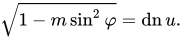
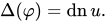
The latter is sometimes called the delta amplitude and is written as

The literature sometimes refers to the complementary parameter, the complementary modulus or the complementary modular angle. They are introduced as follows:

• — the complementary parameter;
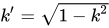• — the complementary modulus;
• — the complementary modular angle.

The Legendre normal elliptic integral of the 1st kind F is defined as

,

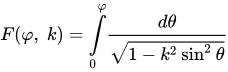or, in Jacobi's form,

.

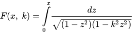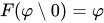
The notation for elliptic integrals is not universally accepted. One must distinguish separators between the variable and the parameter such as "\", "|" and ",". Where a vertical bar is used as the separator, the parameter of the integral follows it, whereas after a backslash comes the modular angle. In particular, the following relation holds

.

;

;

;

;

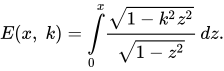
The Legendre normal elliptic integral of the 2nd kind E is defined as

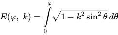
or, using the substitution x=sin⁡φ,

E(φ,0)=φ ;

E(iφ,0)=iφ ;

E(φ,1)=sin⁡φ ;

E(iφ,1)=i sh ⁡φ .

The Legendre normal elliptic integral of the 3rd kind Π is defined as

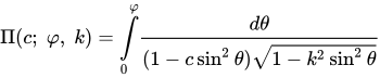
or

The number c is called the characteristic and can take any value, independently of the other arguments. The properties of the elliptic integral of the 3rd kind depend essentially on the value of the characteristic. Note that the value of the integral tends to infinity for any m.

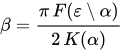
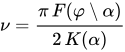
Let us introduce additional notation:

;

;

;

;

;

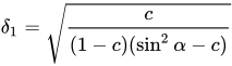K(α) — the complete Legendre normal elliptic integral of the 1st kind.

Then the integral can be written in terms of the Jacobi theta functions:

where

and

By means of the substitution this case reduces to the previous one, since

Let us additionally introduce the quantity

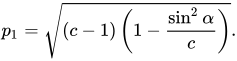
Then:

Let us introduce additional notation:

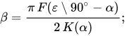
q=q(α);

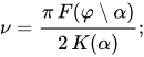
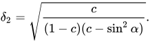
Then the elliptic integral is equal to:

where

and

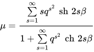
By means of the substitution 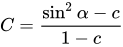this case reduces to the previous one, since

Let us additionally introduce the quantity

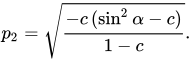
Then:

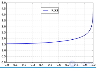
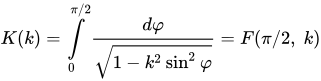
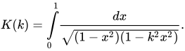
If the amplitude φ of the Legendre normal elliptic integral of the 1st kind is equal to π/2, it is called the complete Legendre normal elliptic integral of the 1st kind:

or

The complete elliptic integral of the 1st kind can be represented as a power series:

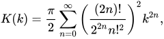
which is equivalent to the expression

where n!! denotes the double factorial.

The complete elliptic integral of the 1st kind can be written in terms of the hypergeometric function as follows:

.

.

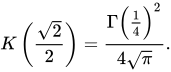
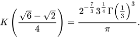
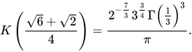
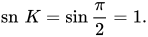
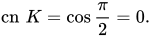
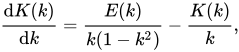
where E(k) is the complete Legendre normal elliptic integral of the 2nd kind, defined in the next section.

The complete elliptic integral of the 1st kind is a solution of the differential equation

The second solution of this equation is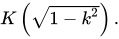

If the amplitude φ of the Legendre normal elliptic integral of the 2nd kind is equal to π/2 , it is called the complete Legendre normal elliptic integral of the 2nd kind:

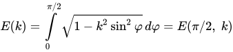
or

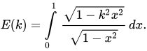
The complete elliptic integral of the 2nd kind can be represented as a power series:

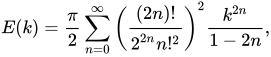
which is equivalent to the expression

The complete elliptic integral of the 2nd kind can be written in terms of the hypergeometric function as follows:

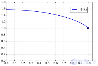
E(1)=1.

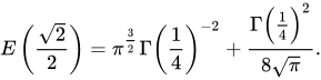
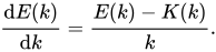
The complete elliptic integral of the 2nd kind is a solution of the differential equation

The second solution of this equation is the function

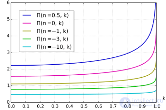
By analogy with the complete elliptic integrals of the 1st and 2nd kind, one can introduce the complete elliptic integral of the 3rd kind:

or

,

where is the Jacobi zeta function.

where is the Heuman lambda function.

or

Practical applications of elliptic integrals

Elliptic integrals are not just abstract mathematics. They arise naturally in many real physical, geometric and engineering problems. Below is a brief but systematic overview:

1. Geometry and arc lengths

The classical origin of elliptic integrals is the computation of the perimeter of an ellipse.

Example:

The perimeter of an ellipse with semi-axes a,ba, ba,b:

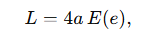
where 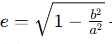is the eccentricity,
and E(e) is the elliptic integral of the second kind.

The perimeter of an ellipse cannot be expressed in terms of elementary functions, only in terms of elliptic ones.

2. Physics of oscillations and pendulums

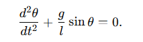
A real (not small!) simple pendulum is described by the equation:

The solution is expressed through the inverse Jacobi elliptic functions (and the period through K(k) ):

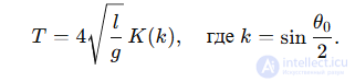
That is, at large amplitudes the period of the pendulum increases, and the formula 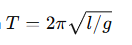becomes inaccurate.

3. Electrodynamics, magnetic fields, potentials

In problems of computing mutual inductance, the field of a circular current, and eddy currents, elliptic integrals describe:

• the magnetic field on the axis of a ring,

• the flux through a loop,

• the inductance between coaxial rings.

For example, for a circular conductor of radius aaa and an observer at distance rrr:

where k depends on the geometry.

4. Mechanics, orbits and celestial mechanics

Elliptic integrals appear in:

• computing trajectories under inverse-square forces (orbits, gravity);

• calculations of the time of motion along an orbit;

• modeling precession and nutation.

5. Potential theory, surface integrals

When solving integrals of the type:

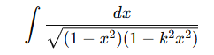
or when parametrizing elliptic cylinders and quadric surfaces.

6. Electronics and signals

In filter theory:

• Elliptic filters (Cauer filters) are named precisely because of the connection of their amplitude response with the Jacobi elliptic functions.

• The formulas for calculating filter parameters include K(k) and E(k).

7. Modern computational and graphics applications

• in modeling deformations (anisotropic surfaces);

• in generating elliptical contours and surfaces in 3D graphics;

• in the analytic geometry of second-order curves.

8. Pure mathematics

Elliptic integrals and their inverse functions (Jacobi and Weierstrass functions) are the foundation of elliptic curves, on which the following are based:

• modern cryptography (ECC),

• number theory (modular forms, the Fermat–Weil–Tate theorem).

• [[b13669]]
• Elliptic curve
• Special functions
• Approximations of elliptic integrals