
Lecture 72 min.
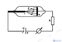
The miniaturization of electron vacuum tubes led to the abandonment of heated cathodes and a transition to field electron emission from cold cathodes of special shape made of specially selected materials[3]. This makes it possible to bring device dimensions down to the micron scale and to use standard semiconductor-industry process technologies in their fabrication[4]. Such designs are currently being actively researched.
Field electron emission , also known as field-induced electron emission, field emission ( FE ) and electron field emission , is the emission of electrons from a material placed in an electrostatic field . The most common example is field emission from a solid surface into vacuum . However, field emission can occur from solid or liquid surfaces, into vacuum, a fluid (e.g. air ) or any nonconducting or weakly conducting dielectric . The field-induced promotion of electrons from the valence band to the conduction band of semiconductors ( the Zener effect ) can also be regarded as a form of field emission.
Field emission in pure metals occurs in high electric fields : the gradients are typically above 1 gigavolt per metre and strongly dependent on the work function . Although field-emission-based electron sources have a number of applications, field emission is most often an undesirable primary source of vacuum breakdown and electrical discharge phenomena, which engineers work to prevent. Examples of applications of surface field emission are the creation of bright electron sources for high-resolution electron microscopes or the discharge of induced charges from spacecraft . Devices that eliminate induced charges are called charge neutralizers .
Historically, the phenomenon of field electron emission has been known under various names, including the "aeona effect", "autoelectronic emission", "cold emission", "cold cathode emission", "field emission", "field electron emission" and "electron field emission". In some contexts (for example, in space engineering) the name "field emission" is applied to field-induced ion emission (field ion emission) rather than to electrons, and because in some theoretical contexts "field emission" is used as a general name covering both field electron emission and field ion emission.
In the late 1920s, field emission was explained by the quantum tunnelling of electrons. This became one of the triumphs of the emerging quantum mechanics . The theory of field emission from bulk metals was proposed by Ralph H. Fowler and Lothar Wolfgang Nordheim . [ 1 ] A family of approximate equations, the Fowler–Nordheim equations , is named after them. Strictly speaking, the Fowler–Nordheim equations apply only to field emission from bulk metals and (with appropriate modifications) to other bulk crystalline solids , but they are often used – as a rough approximation – to describe field emission from other materials.
The related phenomena of the surface photoelectric effect, thermionic emission (or the Richardson–Dushman effect ) and "cold electron emission", that is, the emission of electrons in strong static (or quasi-static) electric fields, were discovered and studied independently from the 1880s to the 1930s. In the modern context, cold field electron emission (CFE) is the name of a particular statistical emission regime in which the electrons in the emitter are initially in internal thermodynamic equilibrium , and in which most emitted electrons escape the emitter by Fowler–Nordheim tunnelling from electron states close to the emitter Fermi level . (By contrast, in the Schottky emission regime, most electrons escape over a field-lowered barrier from states well above the Fermi level.) Many solid and liquid materials can emit electrons in the CFE regime if an electric field of appropriate magnitude is applied. When the term " field emission" is used without qualification, it usually means "cold emission".
For metals, the CFE regime extends well above room temperature. There are other regimes of electron emission (such as " thermal electron emission " and " Schottky emission ") that require significant external heating of the emitter. There are also emission regimes in which the internal electrons are not in thermodynamic equilibrium, and the emission current is partly or wholly determined by the supply of electrons to the emitting region. Such a non-equilibrium emission process can be called field (electron) emission if most of the electrons escape by tunnelling, but strictly speaking it is not CFE, and it cannot be accurately described by a Fowler–Nordheim-type equation.
The equations in this article are written using the modern International System of Quantities (ISQ). Earlier work on field emission (and articles that copy equations directly from older work) often uses Gaussian units, so that the physical constant ε₀ is omitted . In this article all such equations have been converted to the modern international form.
Because the work function is usually expressed in electronvolts (eV), and it is often convenient to use volts per nanometre (V/nm) as the unit of field, this is increasingly becoming standard practice in field emission research. The numerical values of universal constants given here are written in units derived from eV, V and nm, and are calculated to seven significant figures using the 2006 values of the fundamental constants.
In retrospect, it seems likely that the electrical discharges reported by J. H. Winkler [ 2 ] in 1744 were caused by CFE from his wire electrode. However, meaningful research had to wait until the identification of the electron by J. J. Thomson [ 3 ] in 1897 and until it became understood – from work on thermal emission [ 4 ] and photoemission [ 5 ] – that electrons can be emitted from inside metals (rather than from surface-adsorbed gas molecules ), and that – in the absence of applied fields – electrons leaving metals must overcome the work function barrier.
As early as 1913, there was a suspicion that field-induced emission is a distinct physical effect. [ 6 ] However, this suggestion gained wide acceptance only after significant improvements in vacuum technology and sample-cleaning methods. Lilienfeld (who was mainly interested in electron sources for medical X-ray studies) published in 1922 [ 7 ] the first clear description in English of the experimental phenomenology of the effect, which he called "autoelectronic emission". He had been working on this subject in Leipzig since about 1910. [ 8 ] [ 9 ]
After 1922, interest in experimental studies grew, especially in the groups led by Millikan at the California Institute of Technology (Caltech) in Pasadena, California [ 10 ] , and Gossling at the General Electric company in London [ 11 ] . Attempts to understand field electron emission included plotting the experimental current–voltage ( i – V ) data in various ways in order to find a linear relationship. The current increased superlinearly with voltage, but plots of log( i ) against V were not straight [ 10 ] . Walter H. Schottky [ 12 ] suggested in 1923 that the effect might be due to thermally induced emission over a field-lowered barrier. If so, plots of log( i ) against √V should be straight, but they were not [ 10 ] . Schottky's explanation is also incompatible with the experimental observation of only a very weak temperature dependence of CFE [ 7 ] – a point that was initially overlooked . [ 6 ]
The breakthrough came when C. C. Lauritsen [ 13 ] (and J. Robert Oppenheimer independently [ 14 ] ) found that plots of log( i ) against 1/ V give good straight lines. This result was published by Millikan and Lauritsen in early 1928. [ 13 ] A theoretical explanation and the original Fowler–Nordheim-type equation appeared shortly afterwards.
Oppenheimer predicted [ 14 ] that field-induced tunnelling of electrons out of atoms (an effect now called field ionization) would have this i ( V ) dependence, found this dependence in the published field emission results of Millikan and Eyring [ 10 ] and proposed that CFE is due to field-induced tunnelling of electrons from atom-like orbitals on surface metal atoms. The alternative theory of Fowler – Nordheim [ 1 ] theory assumed field-induced tunnelling from free-electron-like states in what we now call the metallic conduction band , with the electron states occupied according to Fermi–Dirac statistics . The Fowler–Nordheim theory explained both the Millikan–Lauritsen result and the very weak temperature dependence of the current.
Serious errors were made in the mathematical details of Oppenheimer's theory. [ 15 ] A small numerical error was also made in the final equation given in the Fowler–Nordheim theory for the CFE current density , which was corrected in a 1929 paper. [ 16 ] If the barrier field in the 1928 Fowler–Nordheim theory is exactly proportional to the applied voltage, and if the emission area is independent of voltage, then the 1928 Fowler–Nordheim theory predicts that plots of log( i / V 2 ) against 1/ V should be exact straight lines. However, the experimental techniques of the time did not allow the Fowler–Nordheim theoretical result to be distinguished from the Millikan–Lauritsen experimental result.
In the physics literature, the work of Fowler and Nordheim is often presented as proof of the tunnelling of electrons predicted by wave mechanics. While this is true, wave mechanics was largely accepted by 1928. Instead, the Fowler–Nordheim work was more revolutionary in establishing the modern theory of electronic bands . Before 1928, it was hypothesized that metals contain two types of electrons, "thermions" and "conduction electrons", and that thermally emitted electron currents are due to the emission of thermions, while field-emitted currents are due to the emission of conduction electrons; only in 1927 did Sommerfeld argue that Fermi–Dirac statistics apply to the behaviour of electrons in metals. [ 17 ] The 1928 Fowler–Nordheim work showed that thermions need not exist as a separate class of internal electrons: electrons can originate from a single band occupied according to Fermi–Dirac statistics, but are emitted in statistically different ways under different conditions of temperature and applied field. The success of the Fowler–Nordheim theory largely confirmed the correctness of Sommerfeld's ideas. [ 18 ]
In particular, the original Fowler–Nordheim-type equation was one of the first to incorporate the statistical-mechanical consequences of the existence of electron spin into the theory of an experimental condensed-matter effect. The Fowler–Nordheim work also laid the physical foundation for a unified approach to field-induced and thermally induced electron emission . [ 18 ]
The ideas of Oppenheimer , Fowler and Nordheim also served as an important stimulus for the development by George Gamow [ 19 ] , and also by Ronald W. Gurney and Edward Condon [ 20 ] [ 21 ] later , in 1928, of the theory of radioactive decay of nuclei (by tunnelling of alpha particles ). [ 22 ]
As already noted, early experimental work on field electron emission (1910–1920) [ 7 ] was motivated by the wish of Lilienfeld to develop miniature X-ray tubes for medical applications. However, it was still too early for this technology to succeed. [ Why? ]
Following the theoretical work of Fowler and Nordheim in 1928, significant progress was made with the development in 1937 by Erwin W. Müller of the spherical field electron microscope (FEM) [ 23 ] (also called the "field emission microscope"). In this instrument the electron emitter is a pointed wire with a tip radius r . It is placed in a vacuum chamber opposite an image detector (originally a phosphor screen) at a distance R from it. The microscope screen shows a projection image of the distribution of current density J over the emitter tip, with a magnification of approximately ( R / r ), typically 10⁵ to 10⁶ . In FEM studies the tip radius is typically from 100 nm to 1 μm. The tip of the pointed wire, when referred to as a physical object, is called a "field emitter", a "tip" or (more recently) a "Müller emitter".
When the emitter surface is clean, the FEM image obtained is characterized by the following:
In the FEM image, dark regions correspond to areas where the local work function φ is relatively high and/or the local barrier field F is relatively low, so that J is relatively low; bright regions correspond to areas where φ is relatively low and/or F is relatively high, so that J is relatively high. This is consistent with the predictions of the exponent of Fowler–Nordheim-type equations [see equation (30) below].
Adsorption of layers of gas atoms (such as oxygen) on the emitter surface or part of it can create surface electric dipoles , which change the local work function of that part of the surface. This affects the FEM image; in addition, the change in work function can be measured using a Fowler–Nordheim plot (see below). FEM thus became one of the first observational tools in surface science . [ 24 ] [ 25 ] For example, in the 1960s FEM results contributed significantly to discussions of heterogeneous catalysis . [ 26 ] FEM was also used to study surface diffusion of atoms . However, FEM has now been almost completely superseded by newer surface-science techniques.
A consequence of the development of FEM and of subsequent experiments was that it became possible to determine (from analysis of FEM images) when an emitter is "clean" and therefore exhibits the work function of a clean surface established by other methods. This was important in experiments designed to test the validity of the standard Fowler–Nordheim-type equation. [ 27 ] [ 28 ] In these experiments the value of the voltage-to-barrier-field conversion factor β was derived from a Fowler–Nordheim plot (see below), assuming a value of φ for a clean surface of tungsten, and compared with values obtained from observations of the emitter shape using an electron microscope and from electrostatic modelling. Agreement to within 10% was achieved. Only quite recently [ 29 ] has it become possible to make the comparison in the reverse direction, by bringing a well-prepared probe so close to a well-prepared surface that an approximate parallel-plate geometry can be assumed and the conversion factor can be taken as 1/ W , where W is the measured probe-to-emitter distance. Analysis of the resulting Fowler–Nordheim plot yields a work function value close to the independently known work function of the emitter.
Measurements of the energy distribution of field-emitted electrons were first published in 1939. [ 30 ] In 1959 Young realized theoretically [ 31 ] and Young and Müller confirmed experimentally [ 32 ] that the quantity measured in spherical geometry is the distribution of the total energy of the emitted electron (its "total energy distribution"). This is because in spherical geometry the electrons move in such a way that the angular momentum about a point in the emitter is approximately conserved. Consequently, any kinetic energy that at emission is directed parallel to the emitter surface is converted into energy associated with the radial direction of motion. Thus the total energy at emission is what is measured in the energy analyser.
With the advent of sensitive electron energy analysers in the 1960s, it became possible to measure the finest details of the total energy distribution. These details reflect the subtleties of surface physics , and the technique of field electron spectroscopy flourished for a time before being displaced by newer surface-investigation methods. [ 33 ] [ 34 ]
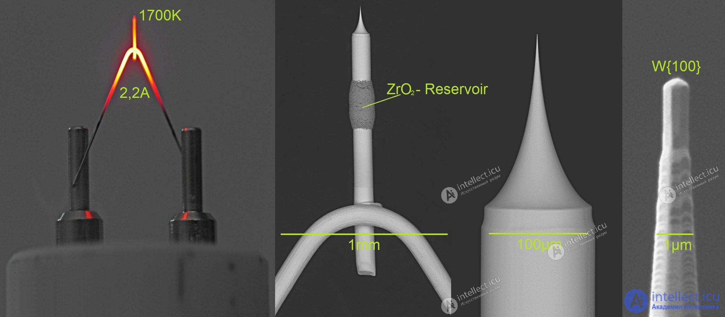
To achieve high resolution in electron microscopes and other electron-beam instruments (such as those used for electron-beam lithography) it is useful to start with an electron source that is small, optically bright and stable. Sources based on the Müller emitter geometry meet the first two criteria well. The first observation of a single atom in an electron microscope (EM) was made by Albert Crewe , J. Wall and J. Langmore in 1970 [ 35 ] using a scanning transmission electron microscope, equipped with an early field emission gun .
Beginning in the 1950s, considerable effort was devoted to developing field emission sources for use in electron guns . [ 36 ] [ 37 ] [ 38 ] [e.g. DD53] Methods were developed for generating axial beams either by build-up of the emitter under the action of the field, or by selective deposition of an adsorbate with a low work function (usually zirconium oxide – ZrO) on the flat tip of a tungsten emitter, oriented along the (100) plane . [ 39 ]
Sources operating at room temperature have the disadvantage that they can become covered with adsorbate molecules arriving from the walls of the vacuum system, and the emitter has to be cleaned from time to time by "flashing" it to a high temperature. Sources based on Müller emitters operating at elevated temperatures, either in the Schottky emission regime or in the so-called intermediate temperature-field regime, are now widely used. Most modern high-resolution electron microscopes and electron-beam instruments use some form of field electron emission source. Attempts are currently being made to develop carbon nanotubes (CNTs) as field emission sources for electron guns. [ 40 ] [ 41 ]
The use of field emission sources in electron-optical instruments required the development of appropriate theories of charged-particle optics [ 37 ] [ 42 ] and the development of suitable models. Various shape models have been tried for Müller emitters; the best appears to be the "sphere on orthogonal cone" (SOC) model proposed by Dyke, Trolan, Dolan and Barnes in 1953 [ 43 ]. Important simulations involving trajectory tracing using the SOC emitter model were carried out by Wiesener and Everhart [ 44 ] [ 45 ] [ 46 ] . The ability to simulate field emission from Müller emitters is now often included in commercial electron-optics software used to design electron-beam instruments. Designing effective modern field emission electron guns requires highly specialized knowledge.
Very sharp emitters can now be produced, including emitters that terminate in a single atom. In this case, electron emission comes from a region roughly twice the crystallographic size of a single atom. This was demonstrated by comparing images of the emitter obtained with a field electron microscope (FEM) and a field ion microscope (FIM). [ 47 ] Müller emitters with a single-atom apex are also relevant to scanning probe microscopy and scanning helium ion microscopy (He SIM). [ 48 ] Methods for producing them have been studied for many years. [ 47 ] [ 49 ] An important recent development has also been an automated technique (for use in He SIM) for restoring a three-atom apex (a "trimer") to its original state if the trimer breaks up. [ 48 ]
Large-area field emission sources have been of interest since the 1970s. In these devices, a high density of individual field emission sites is created on a substrate (originally silicon). This area of research was called first "vacuum microelectronics" and is now called "vacuum nanoelectronics".
One of the two original types of device, the "Spindt array" [ 50 ], used fabrication methods from silicon integrated circuits (ICs) to create regular arrays in which molybdenum cones were deposited in small cylindrical voids in an oxide film, with the void capped by a counter-electrode with a central circular hole. This general geometry has also been used with carbon nanotubes grown in the void.
The other original type of device is the "Latham emitter". [ 51 ] [ 52 ] These were MIMIV (metal-insulator-metal-insulator-vacuum) devices, or, more generally, CDCDV (conductor-dielectric-conductor-dielectric-vacuum) devices, containing conducting particles in a dielectric film. The device emits field electrons because its microstructure/nanostructure has field-enhancing properties. This material had a potential manufacturing advantage, because it could be applied as an "ink", so IC fabrication methods were not needed. In practice, however, it proved difficult to make devices with uniform reliability.
Research has moved on to look for other materials that can be deposited/grown as thin films with suitable field-enhancing properties. In a parallel-plate configuration, the "macroscopic" field F M between the plates is given by F M = V / W , where W is the plate separation and V is the applied voltage. If a sharp object is created on one of the plates, then the local field F at its apex will be greater than F M , and can be related to F M by

The parameter γ is called the "field enhancement factor" and is determined mainly by the shape of the object. Because field emission characteristics are determined by the local field F , the higher the value of γ for an object, the lower the value of F M at which significant emission occurs. Consequently, for a given value of W , the lower the applied voltage V, the lower the voltage at which significant emission occurs.
For about ten years, beginning in the mid-1990s, there was great interest in field emission from plasma-deposited films of amorphous and "diamond-like" carbon . [ 53 ] [ 54 ] Interest subsequently declined, partly because of the appearance of emitters based on carbon nanotubes , and partly because of evidence that the emission sites might be associated with carbon particles created in an unknown way during the deposition process : this indicated that quality control in industrial production might be problematic.
The introduction of carbon-nanotube field emitters [ 41 ] in the form of both "mats" and "grown arrays" was a significant step forward. Extensive studies have been made of both their physical characteristics and possible technological applications. [ 40 ] An advantage of carbon nanotubes for field emission is that, because of their high-aspect-ratio shape, they are "natural field-enhancing objects".
In recent years there has also been a significant growth of interest in developing other forms of thin-film emitter, based both on other forms of carbon (such as "carbon nanowalls" [ 55 ] ) and on various forms of wide-bandgap semiconductors [ 56 ] . A particular aim is to develop nanostructures with a "high γ " and a sufficiently high density of individual emission sites. Thin films of nanotubes in the form of nanotube networks are also being used to develop field emission electrodes [ 57 ] [ 58 ] [ 59 ] . It has been shown that, by fine-tuning the fabrication parameters, these networks can reach an optimal density of individual emission sites. [ 57 ] It has been shown that double-layer electrodes, made by depositing two layers of these networks perpendicular to each other, can lower the turn-on electric field (the electric field needed to reach an emission current of 10 μA/cm² ) to 0.3 V/μm and provide stable field emission operation. [ 58 ]
Common problems for all field emission devices, especially those operating in "industrial vacuum" conditions, are that the emission characteristics can deteriorate through adsorption of gas atoms arriving from other parts of the system, and that the emitter shape can in principle be changed for the worse by various unwanted side processes, such as bombardment by ions formed when the emitted electrons collide with gas-phase atoms and/or with the surface of the counter-electrodes. An important industrial requirement is therefore "tolerance of poor vacuum"; this must be taken into account in research on new emitter materials.
At the time of writing, the most promising forms of large-area field emission sources (certainly in terms of the average emission current density achieved) appear to be Spindt arrays and various forms of carbon-nanotube-based sources.
The development of large-area field emission sources was originally driven by the wish to create new, more efficient forms of electronic information display . These are known as "field emission displays" or "nano-emissive displays". Although several prototypes have been demonstrated [ 40 ] , the development of such displays into reliable commercial products has been hampered by a number of industrial manufacturing problems not directly related to the characteristics of the source [En08].
Other proposed applications of large-area field emission sources [ 40 ] include microwave generation , spacecraft neutralization, X-ray generation and (for array sources) multi-beam electron-beam lithography . There are also recent attempts to develop large-area emitters on flexible substrates, in line with the broader trend toward "plastic electronics".
Developing such applications is the task of vacuum nanoelectronics. However, field emitters work best under good ultrahigh-vacuum conditions. Their most successful applications to date (FEM, FES and electron guns) have been achieved under just such conditions. It is regrettable but true that field emitters and industrial vacuum conditions do not go well together, and the associated problems of reliably providing good "vacuum tolerance" for field emission sources used in such conditions still require better solutions (probably more carefully thought-out materials solutions) than those we have now.
As already noted, it is now thought that the earliest manifestations of field electron emission were the electrical discharges caused by it. After the work of Fowler and Nordheim, it became clear that CFE is one of the possible underlying causes of vacuum breakdown and electrical discharge phenomena. (The detailed mechanisms and pathways can be very complex, and there is no single universal cause.) [ 60 ] . Where vacuum breakdown is known to be caused by electron emission from the cathode, the mechanism was initially thought to be CFE from small conducting needle-like protrusions on the surface. Procedures were (and are) used to round and smooth electrode surfaces that could generate unwanted field electron emission currents. However, the work of Latham and others [ 51 ] showed that emission can also be associated with the presence of semiconducting inclusions on smooth surfaces. The physics of emission generation is still not fully understood, but it is suspected that so-called "triple-junction effects" may be involved. Further information can be found in Latham's book [ 51 ] and in the online bibliography. [ 60 ]
In some electronic devices, electron transfer from one material to another or (in the case of tilted bands) from one band to another ("Zener tunneling") takes place by means of a field-induced tunneling process, which can be regarded as a form of Fowler-Nordheim tunneling. For example, Rhoderick's book discusses the theory relating to metal-semiconductor contacts . [ 61 ]
Fowler-Nordheim tunneling is the wave-mechanical tunneling of an electron through an exact or rounded triangular barrier. Depending on the structure of the material, the electron may initially be localized at the surface or delocalized in the bulk and best described by a traveling wave . Emission from the conduction band of a metal is a situation of the second type, which is the only case considered here. The barrier is also assumed to be one-dimensional (i.e., to have no lateral structure) and to have no small-scale structure causing "scattering" or "resonance" effects. These assumptions serve primarily to simplify the theory; however, the atomic structure of matter is effectively ignored.
The treatment consists of four main steps:
The modified equations required for large-area emitters, and issues in the analysis of experimental data, are considered separately.
For an electron, the one-dimensional Schrödinger equation can be written in the form
 |
1 |
where Ψ( x ) — is the wave function of the electron , expressed as a function of the distance x, measured from the electrical surface of the emitter, [ 62 ] ħ is the reduced Planck constant , m is the electron mass, U ( x ) is the potential energy of the electron , E n is the total energy of the electron associated with motion in the x direction, and M ( x ) = [ U ( x ) − E n ] is called the motive energy of the electron. [ 63 ] M ( x ) can be interpreted as the negative of the kinetic energy of the electron associated with the motion of a hypothetical classical point electron in the x direction, and as a positive value in the barrier.
The shape of the tunneling barrier is determined by how M ( x ) varies with position in the region where M ( x ) > 0. In field emission theory, two models have a special place: the exact triangular (ET) barrier , given in ( 2 ); and the Schottky-Nordheim (SN) barrier , given in ( 3 ). [ 64 ] [ 65 ]
 |
2 |
 |
3 |
Here h is the barrier height at zero field (or the zero-field height), e is the elementary positive charge, F is the barrier field, and ε₀ is the electric constant . By convention, F is taken to be positive , although the classical electrostatic field would be negative. The SN equation uses the classical image potential energy to represent the physical effect of "correlation and exchange".
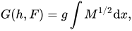
For an electron approaching a given barrier from the inside, the escape probability (or "transmission coefficient" or "penetration coefficient") is a function of h and F and is denoted D ( h , F ) . The main aim of tunneling theory is to calculate D ( h , F ) . For physically realistic barrier models, such as the Schottky-Nordheim barrier, the Schrödinger equation cannot be solved exactly by any simple method. The following so-called "semiclassical" approach can be used. The parameter G ( h , F ) can be defined by means of the JWKB (Jeffreys-Wentzel-Kramers-Brillouin) integral: [ 66 ]
 |
4 |
where the integral is taken across the barrier (i.e., over the region where M > 0), and the parameter g is a universal constant given by
 |
5 |
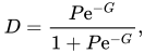
Forbes reformulated a result proved by Fröman and Fröman to show that, formally, in a one-dimensional treatment, the exact solution for D can be written [ 67 ]
 |
6 |
where the tunneling pre-factor P can in principle be calculated by complicated iterative integrations along a path in complex space , but for simple models it is ≈ 1. [ 67 ] [ 68 ] In the CFE regime we have (by definition) G ≫ 1. Equation (6) then reduces to the so-called simple JWKB formula:
 |
7 |
For the exact triangular barrier, substituting equation ( 2 ) into equation ( 4 ) gives G ET = bh 3/2 / F , where
 |
продолжение следует...
Часть 1 Field Electron Emission (Field Emission, Tunnel Emission)
Часть 2 Total energy distribution - Field Electron Emission (Field Emission, Tunnel
Часть 3 Fowler–Nordheim plots and Millikan–Lauritsen plots - Field Electron Emission (Field
Часть 4 Additional theoretical information - Field Electron Emission (Field Emission, Tunnel

Comments