
Lecture 72 min.
Это продолжение увлекательной статьи про автоэлектронная эмиссия.
...
This parameter b is a universal constant, sometimes called the second Fowler-Nordheim constant . For barriers of other shapes we write
 |
9 |
where ν ( h , F ) is a correction factor determined by numerical integration of equation ( 4 ).
The Schottky-Nordheim barrier, which is the barrier model used in deriving the standard Fowler-Nordheim-type equation [ 69 ] , is a special case. In this case, the correction factor is known to be  a function of a single variable f h , defined as f h = F / F h , where F h is the field required to reduce the height of the Schottky-Nordheim barrier from h to 0. This field is given by
 |
10 |
The parameter f h varies from 0 to 1 and can be called the scaled barrier field for a Schottky-Nordheim barrier of zero-field height h .
For the Schottky-Nordheim barrier, ν ( h , F ) is given by the particular value ν ( fh ) of the function ν ( ℓ ′ ). The latter is itself a function of mathematical physics with an explicit series [ 70 ] expansion and is called the principal Schottky-Nordheim barrier function. The following good simple approximation was found for ν ( fh ) : [ 69 ]
 |
11 |
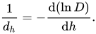
The decay width (in energy), d h , measures how fast the escape probability D decreases as the barrier height h increases; d h is defined as follows:
 |
12 |
When h increases by d h, the escape probability D decreases by a factor close to e ( ≈ 2.718282). For the elementary model based on the exact triangular barrier, where we set ν = 1 and P ≈ 1, we obtain
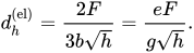
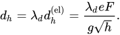
The decay width d h, obtained from the more general expression ( 12 ) differs from this by a "decay-width correction factor" λ d , so that:
 |
13 |
As a rule, the correction factor can be approximately taken as unity.
Of particular interest is the decay width dF for a barrier with h , equal to the local work function φ . Numerically it is given by:
 |
14 |
For metals, the value of dF is typically of the order of 0.2 eV, but varies with the barrier field F.
A historical note is necessary. The idea that the Schottky-Nordheim barrier needs a correction factor, as in equation ( 9 ), was proposed by Nordheim in 1928 [ 65 ] , but his mathematical analysis of the factor was incorrect. A new (correct) function was introduced by Burgess, Kroemer and Houston [ 71 ] in 1953, and its mathematical development was continued by Murphy and Good in 1956 [ 72 ]. This corrected function, sometimes known as the "special field emission elliptic function", was expressed as a function of the mathematical variable y, known as the "Nordheim parameter". Only recently (from 2006 to 2008) has it become clear that it is mathematically much better to use the variable ℓ ′ (= y² ) . And only recently has it become possible to complete the definition of ν ( ℓ ′ ) by developing and proving the validity of an exact series expansion for this function (starting from known special-case solutions of Gauss's hypergeometric differential equation ). The approximation ( 11 ) has likewise been found only recently. Approximation ( 11 ) is superior to, and presumably will eventually supersede, all older approximations of equivalent complexity. These recent developments and their consequences are likely to have a significant effect on field emission research in due course.
The following summary brings these results together. For tunneling well below the top of a well-behaved barrier of reasonable height, the escape probability D ( h , F ) is formally given as follows:
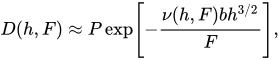 |
15 |
where ν ( h , F ) is a correction factor that in general must be found by numerical integration. For the special case of the Schottky-Nordheim barrier there is an analytical result, and ν ( h , F ) is given as ν ( fh ), as discussed above; approximation (11) for ν ( fh ) is more than adequate for all technological purposes. The pre-factor P is also in principle a function of h and (possibly) F , but for the simple physical models discussed here , it is usually sufficient to make the approximation P = 1. The exact triangular barrier is a special case in which the Schrödinger equation can be solved exactly, as was done by Fowler and Nordheim; [ 1 ] for this physically unrealistic case ν ( fh ) = 1 , and there is an analytical approximation for P.
The approach described here was originally developed to describe Fowler-Nordheim tunneling from smooth, classically flat, planar emitting surfaces. It is suitable for smooth, classically curved surfaces with radii down to 10-20 nm. It can be adapted to surfaces with a sharper radius, but then quantities such as ν and D, become significant functions of the parameter(s) used to describe the surface curvature. When the emitter is so sharp that atomic-level details cannot be neglected, and/or the tunneling barrier is thicker than the dimensions of the emitter apex, a more sophisticated approach is desirable.
As noted at the beginning, in the relatively simple descriptions of field electron emission discussed here, the influence of the atomic structure of materials is ignored. Correct treatment of atomic structure is a very difficult problem, and only limited progress has been made. [ 33 ] However, it is likely that the main effect on Fowler-Nordheim tunneling theory will (in essence) be to change the values of P and ν in equation (15) by amounts that are currently difficult to estimate.
All these remarks in principle apply to Fowler-Nordheim tunneling from any conductor where (before tunneling) the electrons can be regarded as being in traveling-wave states . This approach can be adapted to apply (approximately) to situations where the electrons are initially in localized states on or very close to the emitting surface, but that is beyond the scope of this article.
The energy distribution of the emitted electrons is important both for scientific experiments that use the energy distribution of emitted electrons to investigate aspects of emitter surface physics [ 34 ] , and for field emission sources used in electron-beam instruments such as electron microscopes [ 42 ] . In the latter case, the "width" (in energy) of the distribution affects how sharply the beam can be focused.
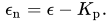
The theoretical explanation here follows Forbes' approach. [ 73 ] If ε denotes the total energy of an electron relative to the emitter Fermi level, and Kp denotes the kinetic energy of the electron parallel to the emitter surface, then the electron's normal energy εn ( sometimes called its "forward energy") is defined as follows:
 |
16 |
Two types of theoretical energy distribution are distinguished: the normal-energy distribution (NED), which shows, how the energy εn is distributed immediately after emission (i.e., immediately beyond the tunnelling barrier); and the total-energy distribution , which shows how the total energy εn is distributed. When the emitter Fermi level is used as the zero reference level, both εn , and εn can be either positive or negative.
Energy-analysis experiments have been carried out on field emitters since the 1930s. However, only in the late 1950s (by Young and Müller [ 31 ] [,YM58]) did it become clear that these experiments always measured the total-energy distribution, now usually denoted by j ( ε ). This is also true (or nearly true) when emission comes from a small field-enhancing protrusion on a flat surface. [ 34 ]
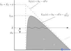
To understand how the total-energy distribution can be calculated within the Sommerfeld free-electron model , consider the PT energy-space diagram (PT="parallel-total").
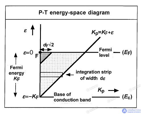
In the diagram, the horizontal axis shows the "parallel kinetic energy" Kp , and the vertical axis shows the total energy ε . An electron inside the bulk metal typically has values of Kp and ε , that lie within the lightly shaded region. It can be shown that each element dεdKp in this energy space makes a contribution .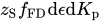 to the density of the electron current incident on the inner boundary of the emitter. [ 73 ] Here z S is a universal constant (here called the Sommerfeld supply density ):
 |
17 |
and is the Fermi–Dirac distribution function :
 |
18 |
where T is the thermodynamic temperature , and kB is the Boltzmann constant .
This element of incident current density encounters a barrier of height h, given by:
 |
19a |
The corresponding escape probability is D ( h , F ) : it can be expanded (approximately) in the form [ 73 ]
 |
19b |
where D F is the escape probability through a barrier of unreduced height equal to the local work function φ . Consequently, the element d ε d K p makes a contribution  to the emission current density, and thus the total contribution from incident electrons with energies in the elementary range dε is
 |
20 |
where the integral is in principle taken along the strip shown in the diagram, but in practice can be extended to ∞ when the decay width dF is much smaller than the Fermi energy KF ( which always holds for a metal). The result of the integration can be written as follows:
 |
21 |
where and
 are the values appropriate for a barrier of unreduced height h, equal to the local work function
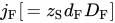 is defined by this equation.
For a given emitter to which a given field is applied, is independent of F , so equation (21) shows that the shape of the distribution (as ε increases from a negative value well below the Fermi level) is a rising exponential multiplied by the FD distribution function. This gives rise to the familiar distribution shape, first predicted by Young. [ 31 ] At low temperatures,
 near the Fermi level the value falls sharply from 1 to 0, and the full width of the distribution at half maximum (FWHM) is given by:
 |
22 |
The fact that experimental CFE total-energy distributions have this basic shape is good experimental confirmation that electrons in metals obey Fermi–Dirac statistics .
Fowler–Nordheim-type equations in the J – F form are (approximate) theoretical equations derived to describe the local current density J, emitted from the internal electron states in the conduction band of a bulk metal. The emission current density (ECD) J for some small uniform region of the emitting surface is usually expressed as a function J ( φ , F ) of the local work function φ and the local barrier field F that characterize this small region. For sharply curved surfaces, J may also depend on the parameter(s) used to describe the surface curvature.
Because of the physical assumptions made in the original derivation [ 1 ] , the term "Fowler–Nordheim-type equation" was for a long time used only for equations describing ECD at zero temperature. However, it is better to allow this name to be used for slightly modified equations (discussed below) that are valid for finite temperatures in the CFE emission regime.
Current density is best measured in A/m² . The total current density emitted from a small uniform region can be obtained by integrating the total-energy distribution j ( ε ) over the total electron energy ε . At zero temperature the Fermi–Dirac distribution function fFD = 1 for ε < 0 and fFD = 0 for ε > 0. Thus , the ECD at 0 K, J0 , is determined from equation (18) as follows :
 |
23 |
where 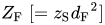 is the effective supply for state F and is defined by this equation. Strictly speaking, the lower limit of the integral should be − K F , where K F is the Fermi energy ; but if d F is much smaller than K F (which always holds for a metal), then energies below K F make no significant contribution to the integral, and it can formally be extended to –∞.
Result (23) can be interpreted simply and usefully in physical terms by referring to Fig. 1. The electron state at point "F" in the diagram ("state F") is the "forward-moving state at the Fermi level" (i.e., it describes a Fermi-level electron moving perpendicular to the emitter surface). At 0 K, an electron in this state sees a barrier of unreduced height φ and has an escape probability D F , which is higher than that of any other occupied electron state. It is therefore convenient to write J 0 as Z F D F , where the "effective supply" Z F is the current density that state F would have to carry inside the metal if all the emission came from state F.
In practice, the current density is mainly built up from a group of states close in energy to state F, most of which lie in the heavily shaded region of the energy-space diagram. Since, for the free-electron model , the contribution to the current density is directly proportional to the area in energy space (with the Sommerfeld supply density z S as the proportionality coefficient), it is useful to regard the ECD as the result of electron states being formed in a region of size d F 2 (measured in eV 2 ) on the energy-space diagram. That is, it is useful to regard the ECD as the result of states being formed in the heavily shaded region in Fig. 1. (This approximation gradually worsens as the temperature rises.)
Z F can also be written in the following form:
 |
24 |
where the universal constant a , sometimes called the first Fowler–Nordheim constant , is given by
 |
25 |
This clearly shows that the pre-exponential factor aφ −1 F 2 , which appears in Fowler–Nordheim-type equations, is related to the effective arrival of electrons at the emitter surface in the free-electron model.
To obtain a result valid for non-zero temperature, note from equation (23) that z S d F D F = J 0 / d F . Thus, when equation (21) is integrated at non-zero temperature, then – making this substitution and inserting the explicit form of the Fermi–Dirac distribution function – the ECD J can be written as:
 |
26 |
where λT is the temperature correction factor , given by the integral. The integral can be transformed by writing 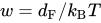 and
 , and then
 into the standard result: [ 74 ]
 |
27 |
This is valid for w > 1 (i.e., d F / k B T > 1 ). Therefore, for temperatures such that k B T < d F :
 |
28 |
where the expansion is valid only if ( π k B T / d F ) ≪ 1. An example value (for φ = 4.5 eV , F = 5 V/nm , T = 300 K ) is λ T = 1.024 . In the CFE regime, λ T is generally considered always to be small compared with other uncertainties, and it is usually not necessary to include it explicitly in current-density formulae at room temperature.
The emission regimes of metals are defined in practice by the ranges of barrier field F and temperature T for which a given family of emission equations is mathematically adequate. When the barrier field F is high enough for the CFE regime to operate for emission from a metal at 0 K, then the condition k B T < d F provides a formal upper (temperature) limit for the CFE emission regime. However, it has been suggested that (because of approximations made elsewhere in the derivation) the condition k B T < 0.7 d F is a better working limit: this corresponds to a value of λ T of about 1.09 and (for the example) an upper temperature limit for the CFE regime of about 1770 K. This limit is a function of the barrier field. [ 33 ] [ 72 ]
Note that result (28) applies here to a barrier of any shape (although d F will differ for different barriers).
Result (23) also makes it possible to understand what happens when atomic-level effects are taken into account and the band structure ceases to resemble that of free electrons. Because of the presence of the atomic ion cores, the surface barrier, as well as the wave functions of electrons at the surface, will be different. This will affect the values of the correction factor , the prefactor P and (to a limited extent) the correction factor λd . These changes will, in turn, affect the values of the parameter D F and (to a limited extent) of the parameter d F. For a real metal, the supply density will vary with position in energy space, and the value at point "F" may differ from the Sommerfeld supply density. We can take this effect into account by introducing an electron band-structure correction factor λB into equation (23). Modinos discussed how this factor can be calculated: he estimates that it is most likely in the range 0.1 to 1; it may fall outside these limits , but is unlikely to fall outside the range 0.01 < λB < 10. [ 75 ]
Defining the overall supply correction factor λ Z as λ T λ B λ d 2 and combining the above equations, we obtain the so-called physically complete Fowler–Nordheim-type equation: [ 76 ]
 |
29 |
where [=( φ , F )] is the correction factor for a barrier of unreduced height φ . This is the most general Fowler–Nordheim-type equation. Other equations of this family are obtained by substituting specific expressions for the three correction factors, P F and λ Z that it contains. The so-called elementary Fowler–Nordheim-type equation, which appears in undergraduate textbooks on field emission, is obtained by substituting λ Z → 1 , P F → 1 ,→ 1 ; this does not give good quantitative predictions, because it makes the barrier stronger than it is in physical reality. The so-called standard Fowler–Nordheim-type equation, originally developed by Murphy and Good [ 72 ] and widely used in the literature of the past, is obtained by substituting λ Z → t F −2 , P F → 1 ,→ v F , where v F is v ( f ), where f is the value of f h, obtained by substituting h = φ , and t F is a related parameter (whose value is close to unity). [ 69 ]
Within the more complete theory described here, the factor t F −2 is an integral part of the correction factor λ d 2 [see [ 67 ] and note that λ d 2 is denoted there as λ D ]. There is no substantial value in continuing to define t F −2 separately. Probably, given the present state of knowledge, the best approximation for modelling CFE from metals on the basis of a simple Fowler–Nordheim-type equation is obtained by substituting λ Z → 1 , P F → 1 ,→ v ( f ) . This restores the Fowler–Nordheim-type equation used by Dyke and Dolan in 1956, and it may be called the "simplified standard Fowler–Nordheim-type equation".
In particular, the recommended simplified standard Fowler–Nordheim-type equation and the corresponding formulae are as follows:
 |
30a |
 |
30b |
 |
30c |
 |
30d |
where F φ here is the field required to reduce to zero the Schottky–Nordheim barrier of unreduced height equal to the local work function φ , and f is the scaled barrier field for a Schottky–Nordheim barrier of unreduced height φ . [This quantity f could be written more precisely as f φ SN , but this makes the Fowler–Nordheim-type equation less cumbersome if the convention is adopted that a plain f means the quantity denoted as f φ SN in [ 69 ] equation (2.16).] For the example ( φ = 4.5 eV , F = 5 V/nm ), f ≈ 0.36 and v ( f ) ≈ 0.58 ; practical ranges for these parameters are discussed further in [ 77 ] .
Note that the variable f (the scaled barrier field) is not the same as the variable y (the Nordheim parameter) widely used in the field emission literature, and that "v ( f )" does NOT have the same mathematical meaning and magnitude as "v ( y )", which appears in the field emission literature. In the context of the revised theory described here, the formulae for v (
продолжение следует...
Часть 1 Field Electron Emission (Field Emission, Tunnel Emission)
Часть 2 Total energy distribution - Field Electron Emission (Field Emission, Tunnel
Часть 3 Fowler–Nordheim plots and Millikan–Lauritsen plots - Field Electron Emission (Field
Часть 4 Additional theoretical information - Field Electron Emission (Field Emission, Tunnel

Comments