
Lecture 72 min.
Это продолжение увлекательной статьи про автоэлектронная эмиссия.
...
y ) and the tables of values for v ( y ) should be ignored or regarded as giving values of v ( f¹ /² ). If more accurate values of v ( f ), then [ 69 ] provides formulae that give values of v ( f ) with an absolute mathematical accuracy better than 8×10⁻¹⁰ . However, the approximation formula (30c) given above, which yields values with an absolute mathematical accuracy better than 0.0025, should give values accurate enough for all technological purposes. [ 69 ]A historical note is needed on the methods of deriving Fowler–Nordheim-type equations. There are several possible approaches to deriving these equations using free-electron theory . The approach used here , was proposed by Forbes in 2004 and can be described as "integration through the total-energy distribution using the parallel kinetic energy Kp as the first integration variable". [ 73 ] Essentially, it is the equivalent of Modinos' procedure [ 33 ] [ 75 ] (in a more advanced quantum-mechanical approach) for free electrons, namely "integration over the surface Brillouin zone". In contrast, the free-electron theory approaches to CFE proposed by Young in 1959 [ 31 ] , Gadzuk and Plummer in 1973 [ 34 ] and Modinos in 1984 [ 33 ] , also integrate through the total-energy distribution, but use the normal energy εn (or a related quantity) as the first integration variable.
There is also an older approach, based on Nordheim's seminal 1928 work [ 78 ] , which formulates the problem differently and then uses first Kp , and then εn (or a related quantity) as the integration variables: this is known as "integration through the normal-energy distribution". This approach continues to be used by some authors. Although it has some advantages, especially when discussing resonance phenomena, it requires integrating the Fermi–Dirac distribution function in the first integration step: for electron band structures unlike those of free electrons, this can lead to very complicated and error-prone mathematics (as in Stratton's work on semiconductors ) [ 79 ] . Moreover, integration through the normal-energy distribution does not generate the experimentally measured electron energy distributions.
Overall, the approach used here seems more transparent and leads to simpler mathematics.
In principle, it is also closer to the more sophisticated approaches used for real bulk crystalline solids, where the first step is either to integrate the contributions to the current density over surfaces of constant energy in wave-vector space ( k -space) [ 34 ] , or to integrate the contributions over the corresponding surface Brillouin zone [ 33 ] . Forbes's approach is equivalent to either integrating over a spherical surface in k -space, using the variable Kp to define a ring-shaped integration element with cylindrical symmetry about an axis in the direction , perpendicular to the emitting surface, or integrating over the (extended) surface Brillouin zone using circular-ring elements.
The previous section explains how to derive Fowler–Nordheim-type equations. Strictly speaking, these equations apply only to CFE from bulk metals. The ideas presented in the following sections apply to CFE in a more general case, but equation (30) will be used to illustrate them.
For CFE, the basic theoretical calculations establish a relationship between the local emission current density J and the local barrier field F at a local point on the emitting surface. In experiments, one measures the emission current i from some defined part of the emitting surface as a function of the voltage V applied to some counter-electrode. Auxiliary equations are used to relate these variables to J and F .
The voltage-to-barrier-field conversion factor β is defined as follows:
 |
31 |
The value of F varies from point to point on the emitter surface, and the value of β varies accordingly.
For a metallic emitter, the value of β for a given position will be constant (independent of voltage) under the following conditions: (1) the device is a "diode" arrangement, in which the only electrodes present are the emitter and a set of "surrounding" regions, all parts of which are at the same voltage; (2) there is no significant field-emitted vacuum space charge (FEVSC) (this will hold except at very high emission current densities, about 10⁹ A /m² or higher [ 27 ] [ 80 ] ); (3) there are no significant "patch fields" [ 63 ] resulting from local work-function non-uniformities (this is usually assumed to be the case, but in some instances it may not be). For non-metals, the physical effects called "field penetration" and " band bending " [M084] can make β a function of the applied voltage, although – surprisingly – there has been little study of this effect.
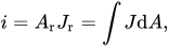
The emission current density J varies from point to point over the emitter surface. The total emission current i from a particular part of the emitter is obtained by integrating J over that part. To obtain a simple equation for i ( V ) the following procedure is used. A reference point "r" is chosen on this part of the emitter surface (often the point at which the current density is a maximum), and the current density at this reference point is denoted by Jr. Then a parameter Ar , called the notional emission area (with respect to point "r"), is defined as follows:
 |
32 |
where the integral is taken over the part of the emitter of interest.
This parameter A r was introduced into CFE theory by Stern, Gossling and Fowler in 1929 (who called it the "weighted mean area"). [ 16 ] For practical emitters, the emission current density used in Fowler–Nordheim-type equations is always the current density at some reference point (although this is usually not stated). A long-established convention denotes this reference current density by the simple symbol J , and the corresponding local field and conversion factor by the simple symbols F and β , without the subscript "r" used above; this convention will be used from here on.
The notional emission area A r will often be a function of the reference local field (and hence of voltage), [ 30 ] and in some cases may be a significant function of temperature.
Because Ar has a mathematical definition, it does not necessarily correspond to the area , from which emission from a point emitter is observed in a field electron (emission) microscope . In the case of a large-area emitter containing many individual emission sites, Ar will almost always be very, very [ clarification needed ] much smaller than the "macroscopic" geometrical area ( AM ) of the emitter, as observed visually (see below).
Incorporating these auxiliary equations into equation (30a) gives
 |
33 |
This is the simplified standard Fowler–Nordheim-type equation in i – V form. The corresponding "physically complete" equation is obtained by multiplying by λ Z P F .
The equations given in the previous section apply to all field emitters operating in the CFE regime. However, further developments are useful for large-area emitters containing many individual emission sources.
For such emitters, the notional emission area will almost always be very, very much smaller than the apparent "macroscopic" geometrical area ( AM ) of the physical emitter, as observed visually. A dimensionless parameter αr, the emission-area efficiency , can be defined as follows:
 |
34 |
One can also define a "macroscopic" (or "average") emission current density J M (averaged over the geometrical area A M of the emitter) and relate it to the reference current density J r used above by the relation
 |
35 |
This leads to the following "large-area versions" of the simplified standard Fowler–Nordheim-type equation:
 |
36 |
 |
37 |
Both of these equations contain the emission-area efficiency factor αr . For any given emitter, the value of this parameter is usually poorly known. In general, αr varies widely depending on the emitter material, and between different samples of the same material , prepared and treated in different ways. Values in the range from 10⁻¹⁰ to 10⁻⁶ , seem likely, and values outside this range are also possible.
The presence of α r in equation (36) explains the difference between the macroscopic current densities often quoted in the literature (typically 10 A/m² for many forms of large-area emitter, other than Spindt arrays [ 50 ] ), and the local current densities at the actual emission sites, which may vary widely, but which are generally thought to be of the order of 10⁹ A /m² or , possibly, somewhat lower.
A significant part of the technological literature on large-area emitters does not clearly distinguish between local and macroscopic current density, or between the notional emission area A r and the macroscopic area A M , and/or omits the parameter α r in the equations quoted. Care is needed to avoid errors of interpretation.
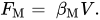
It is also sometimes convenient to separate the conversion factor βr into a "macroscopic part " , which relates to the overall geometry of the emitter and its surroundings, and a "local part", which relates to the ability of the local structure of the emitter surface to enhance the electric field. This is usually done by defining a "macroscopic field" FM , which is the field that would be present at the emission site in the absence of the local structure causing enhancement. This field FM is related to the applied voltage by a "voltage-to-macroscopic-field conversion factor" βM, defined as follows :
 |
38 |
In the typical case of a system consisting of two parallel plates separated by a distance W , on one of which emitting nanostructures have been created, β M = 1/ W .
A "field enhancement factor" γ , is then defined, which is related to the values of βr and βM as follows :
 |
39 |
With the help of equation (31), the following formulas are obtained:
 |
40 |
 |
41 |
where, in accordance with the generally accepted convention, the suffix "r" has now been dropped from parameters relating to the reference point. There are formulas for evaluating γ using classical electrostatics for various emitter shapes, in particular the "hemisphere on a post". [ 81 ]
Equation (40) implies that variants of Fowler–Nordheim-type equations can be written in which either F or βV is everywhere replaced by This is often done in technological applications, where the main interest is in the field enhancement due to the properties of the local emitter nanostructure. However, in some work in the past, the lack of a clear distinction between the barrier field F and the macroscopic field F M has led to confusion or errors.
More generally, the goals of technological development of large-area field emitters are to improve the uniformity of emission by increasing the value of the emission-area efficiency αr and to lower the "turn-on" voltage , at which significant emission occurs, by increasing the value of β . Equation (41) shows that this can be done in two ways: either by trying to develop nanostructures with "high γ ", or by changing the overall geometry of the system so as to increase βM . There are various trade-offs and limitations.
In practice, although the definition of macroscopic field used above is the most common, other (differently defined) types of macroscopic field and field enhancement factor are used in the literature, particularly in connection with the use of probes to investigate the current - voltage characteristics of individual emitters. [ 82 ]
In a technological context, field emission data are often plotted using (a defined value of) F M or 1/ F M as the x coordinate. For scientific analysis, however, it is usually better not to preprocess the experimental data, but to plot directly from the measured i – V data. The values of technological parameters such as (various forms of) γ, can then be obtained from the fitted parameters of the i – V plot (see below), using the appropriate definitions.
Most theoretical derivations in field emission theory are made on the assumption that the barrier has the Schottky–Nordheim form (equation (3)). However, this barrier form is not valid for emitters with radii of curvature R, comparable to the length of the tunneling barrier. The latter depends on the work function and the field, but in cases of practical interest the Schottky–Nordheim barrier approximation can be considered valid for emitters with radii R > 20 nm , as explained in the next paragraph.
The main assumption of the SN barrier approximation is that the electrostatic potential term has a linear form  in the tunneling region. It has been shown that the latter is valid only if
 . [ 83 ] Consequently, if the tunneling region has length
 ,
 for all
 that define the tunneling process; thus, if
 equation (1) is valid, and the SN barrier approximation is acceptable. If the tunneling probability is high enough to cause measurable field emission, L does not exceed 1–2 nm. Consequently, the SN barrier is valid for emitters with radii of the order of several tens of nm.
However, modern emitters are much sharper than this, with radii of the order of a few nanometers. Therefore, the standard FN equation, or any version of it assuming an SN barrier, leads to significant errors for such sharp emitters. This has been shown both theoretically [ 84 ] [ 85 ] , and confirmed experimentally [ 86 ] .
The above problem was solved by Kyritsakis and Xanthakis [ 83 ] , who generalized the SN barrier to include the electrostatic effects of emitter curvature. The general form of the barrier for an emitter with mean radius of curvature  (the reciprocal of the mean of the two principal curvatures) can be asymptotically expanded as [ 87 ]
 . |
43 |
After dropping  terms and using the JWKB approximation (4) for this barrier, the Gamow exponent takes a form that generalizes equation (5)
 |
44 |
where  is defined by formula (30d),
 is given by formula (30c), and
 is a new function that can be approximated similarly to (30c) (typos are corrected in reference [ 83 ] ):
 |
45 |
An expression is given for the Gamow exponent as a function of the zero-field barrier height  . The emission current density for cold field emission can be obtained from equation (23). This gives
 |
46 |
where the functions  and
 are defined as
 |
47a |
and
 |
47b |
In equation (46), for completeness, λ d is not approximated by unity, as it is in (29) and (30a), although for most practical cases this is a very good approximation. In addition, equations (43), (44) and (46) coincide with the corresponding equations of standard Fowler–Nordheim theory (3), (9) and (30a) in the limit R → ∞ ; this is expected, since the former equations generalize the latter.
Finally, it should be noted that the above analysis is asymptotic in the limit L ≪ R , similarly to standard Fowler–Nordheim theory using the SN barrier. However, the addition of quadratic terms makes it significantly more accurate for emitters with radii of curvature in the range ~ 5–20 nm. For sharper emitters there is no general approximation for the current density. To obtain the current density, one must calculate the electrostatic potential and numerically evaluate the JWKB integral . Scientific computing software has been developed for this purpose (see, for example, GETELEC [ 88 ] ).
At this stage in the development of CFE theory, it is important to distinguish between theoretical CFE equations and empirical CFE equations. The former are derived from condensed-matter physics (although in contexts where a detailed description is difficult). An empirical CFE equation, on the other hand, simply attempts to represent the actual experimental form of the dependence of current i on voltage V.
In the 1920s, empirical equations were used to determine the power of V that appeared in the exponent of a semilogarithmic equation that was assumed to describe experimental CFE results. In 1928, theory and experiment were combined to show that (except, perhaps, for very sharp emitters) this power is V −1 . It has recently been suggested that CFE experiments should now be carried out to try to find the power ( κ ) of V in the pre-exponential factor of the following empirical CFE equation: [ 89 ]
 |
48 |
where B , C and κ are treated as constants.
From equation (42) it is easy to show that
 |
49 |
In the 1920s, experimental techniques did not make it possible to distinguish between the results κ = 0 (assumed by Millikan and Lauritsen) [ 13 ] and κ = 2 (predicted by the original Fowler–Nordheim-type equation). [ 1 ] However, it should now be possible to make sufficiently accurate measurements of dlni/d(1/V) (using, if necessary, lock-in detection/phase-sensitive detection techniques and computer-controlled equipment) and to derive κ from the slope of the corresponding plot of the data. [ 50 ]
After the discovery of approximation (30b), it is now quite clear that – even for CFE from bulk metals – a value of κ = 2 is not expected. This can be shown as follows. Using equation (30c) above, the dimensionless parameter η can be defined as follows:
 |
50 |
For φ = 4.50 eV this parameter has the value η = 4.64 . Since f = F / F φ and v ( f ) is given by equation (30b), the exponent in the simplified standard Fowler–Nordheim-type equation (30) can be written in an alternative form and then expanded as follows: [ 69 ]
 |
51 |
Provided that the conversion factor β is independent of voltage, the parameter f has the alternative definition f = V / V φ , where V φ is the voltage required in a particular experimental system to reduce the height of the Schottky–Nordheim barrier from φ to zero. It is thus clear that the factor v ( f ) in the exponent of theoretical equation (30) gives rise to an additional dependence on V in the pre-exponential factor of the empirical equation. Thus (for effects due to the Schottky–Nordheim barrier, and for an emitter with φ = 4.5 eV ) we obtain the prediction:
 |
52 |
Since a voltage dependence may also be observed in a Fowler–Nordheim-type equation in other factors, in particular in the notional emission area [ 30 ] A r and in the local work function, it is not necessarily to be expected that κ for CFE from a metal with a local work function of 4.5 eV will have the value κ = 1.23, but there is certainly no reason to expect it to have the original Fowler–Nordheim value κ = 2. [ 90 ]
The first experimental test of this proposal was made by Kirk, who used a somewhat more complicated form of data analysis to find a value of 1.36 for his parameter κ . His parameter κ is very similar to the parameter κ, used here, but not quite identical to it, although his results seem to confirm the potential usefulness of this form of analysis. [ 91 ]
Using the empirical CFE equation (42) and measuring κ may be particularly useful for non-metals. Strictly speaking, Fowler–Nordheim-type equations apply only to emission from the conduction band of bulk crystalline solids. However, empirical equations of the form (42) should apply to all materials (although modification may perhaps be needed for very sharp emitters). It is quite likely that one of the differences between CFE equations for new materials and Fowler–Nordheim-type equations is that these CFE equations may have a different power of F (or V ) in their pre-exponential functions. Measurements of κ may provide some experimental confirmation of this.
The original theoretical equation derived by Fowler and Nordheim [ 1 ] , has over the last 80 years influenced the way in which experimental CFE data are plotted and analyzed. In the widely used Fowler–Nordheim plot, introduced by Stern et al. in 1929 [ 16 ] , the quantity ln{ i / V² } is plotted against 1/ V . It was originally assumed that (as predicted by the original or elementary Fowler–Nordheim-type equation) this would produce an exact straight line with slope S FN . S FN would be related to the parameters that appear in the exponent of the Fowler–Nordheim-type equation of i – V- form, as follows:
 |
47 |
Consequently, knowledge of φ would make it possible to determine β , or vice versa.
In principle, in systems whose geometry contains a local field-enhancing nanostructure, and for which a macroscopic conversion factor can be defined, β M , knowledge of β makes it possible to determine the value of the effective field enhancement factor of the emitter γ by the formula γ = β / β M. In the usual case of a film emitter formed on one plate of a two-plate system with a plate separation W (so that β M = 1/ W ), then
 |
48 |
At present this is one of the most likely applications of Fowler–Nordheim plots.
It subsequently became clear that the original explanation given above is strictly valid only for the physically unrealistic situation of a planar emitter and a triangular barrier. For real emitters and barriers, it is necessary to introduce a "slope correction factor" σ FN , which leads to a revised formula.
 |
49 |
In principle, the value of σ FN will depend on any parameter in a physically complete Fowler–Nordheim-type equation for i ( V ) that has a voltage dependence.
At present the only parameter considered important is the correction factor  relating to the barrier shape, and the only barrier for which any well-developed detailed theory exists is the Schottky–Nordheim barrier. In this case σ FN is given by a mathematical function called s . This function s was first correctly presented in tabular form (as a function of the Nordheim parameter y ) by Burgess, Kroemer and Houston in 1953; [ 71 ] and a modern treatment giving s as a function of the scaled barrier field f for the Schottky–Nordheim barrier is given in [ 69 ] . However, it has long been clear that for practical emitter work the value of s lies in the range 0.9 to 1.
In practice, because of the additional complexity involved in accounting in detail for the slope correction factor, many authors (in effect) substitute σ FN = 1 into equation (49), thereby introducing a systematic error into their estimated values of β and/or γ , which is usually considered to be around 5%.
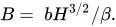
However, the empirical equation (42) – which is in principle more general than Fowler–Nordheim-type equations – opens up new possibilities for analysing field emission i – V data. In general one can assume that the parameter B in the empirical equation is related to the irreducible height H of some characteristic barrier experienced by the tunnelling electrons.
 |
50 |
(In most cases, but not necessarily all, H will equal the local work function; this is certainly true for metals.) The question is how to determine the value of B experimentally. There are two obvious ways. (1) Assume that equation (43) can be used to obtain a sufficiently accurate experimental value of κ from the slope of a plot of the form [−dln{ i }/d(1/ V ) versus V ]. In this case a second plot of ln( i )/ V κ versus 1/ V should be an accurate straight line with slope − B . This approach should be the most accurate way of determining B.
(2) Alternatively, if the value of κ is not accurately known and cannot be accurately measured, but can be estimated or assumed, then the value of B can be obtained from a plot of the form [ln{ i } vs. 1/ V ]. This is the form of plot used by Millikan and Lauritsen in 1928. Rearranging equation (43) gives
 |
51 |
Thus B can be determined to a sufficient degree of approximation by finding the average slope of the Millikan–Lauritsen plot over some range of 1/ V values and applying a correction, using the value of 1/ V at the middle of the range and the assumed value of κ .
The main advantages of using a Millikan–Lauritsen plot and this correction procedure over a Fowler–Nordheim plot and a slope correction factor are as follows: (1) The plotting procedure is somewhat simpler. (2) The correction involves a physical parameter ( V ) that is a measurable quantity, rather than a physical parameter ( f ) that must be calculated [in order to subsequently calculate the value of s ( f ) or, more generally, σFN ( f )]. (3) Both the parameter κ , itself and the correction procedure are more transparent (and easier to understand) than the Fowler–Nordheim plot equivalents. (4) This procedure takes into account all the physical effects that influence the value of κ , whereas the Fowler–Nordheim plot correction procedure (in the form in which it has been carried out for the last 50 years) takes into account only those effects that are related to the barrier shape, assuming, moreover, that this shape is a Schottky–Nordheim barrier. (5) There is a clearer separation of theoretical and technological issues: theorists will be interested in establishing what information any measured values of κ provide about CFE theory; but experimentalists can simply use measured values of
продолжение следует...
Часть 1 Field Electron Emission (Field Emission, Tunnel Emission)
Часть 2 Total energy distribution - Field Electron Emission (Field Emission, Tunnel
Часть 3 Fowler–Nordheim plots and Millikan–Lauritsen plots - Field Electron Emission (Field
Часть 4 Additional theoretical information - Field Electron Emission (Field Emission, Tunnel

Comments