Lecture
The artificial neuron ( McCulloc's mathematical neuron, Pitts [en] , the formal neuron [1] ) is a node of an artificial neural network that is a simplified model of a natural neuron. Mathematically, an artificial neuron is usually represented as some non-linear function of a single argument — a linear combination of all input signals. This function is called the activation function [2] or the trigger function , the transfer function . The result is sent to a single output. Such artificial neurons unite in a network - they connect the outputs of some neurons with the inputs of others. Artificial neurons and networks are the main elements of an ideal neurocomputer. [3]
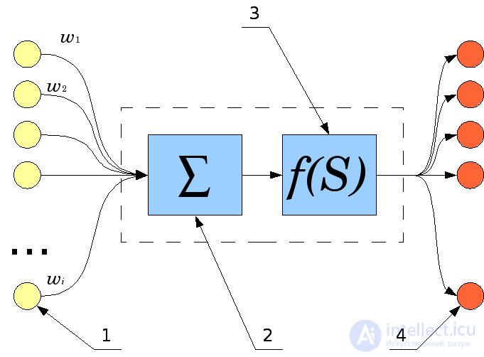
 - weight of input signals
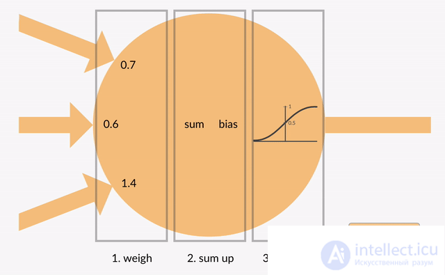
online demonstration of the work of an artificial neuron
A biological neuron consists of a body with a diameter of 3 to 100 microns, containing the nucleus (with a large number of nuclear pores) and other organelles (including a highly developed rough EPR with active ribosomes, the Golgi apparatus), and processes. Allocate two types of shoots. The axon is usually a long process adapted to conduct excitation from the body of a neuron. Dendrites - as a rule, short and highly branched processes, which serve as the main site of formation of excitatory and inhibitory synapses affecting a neuron (different neurons have a different ratio of the length of the axon and dendrites). A neuron can have several dendrites and usually only one axon. One neuron can have connections with 20 thousand other neurons. The human cerebral cortex contains 10–20 billion neurons.
A mathematical model of an artificial neuron was proposed by W. McCulloch and W. Pitts along with a network model consisting of these neurons. The authors showed that the network on such elements can perform numerical and logical operations [4] . In practice, the network was implemented by Frank Rosenblatt in 1958 as a computer program, and later as an electronic device - a perceptron. Initially, a neuron could operate only with signals of a logical zero and a logical unit [5] , since it was built on the basis of a biological prototype, which can exist only in two states - excited or unexcited. The development of neural networks has shown that in order to expand their field of application, it is necessary that the neuron can work not only with binary signals, but also with continuous (analog) signals. Such a generalization of the neuron model was made by Widrow and Hoff [6] , who proposed using the logistic curve as a function of the neuron triggering.
Connections by which the output signals of some neurons arrive at the inputs of others are often called synapses, by analogy with the connections between biological neurons. Each connection is characterized by its weight . Connections with a positive weight are called excitatory , and those with a negative weight are called inhibitory [7] . A neuron has one way out, often called an axon, by analogy with a biological prototype. With a single output of the neuron, the signal can be sent to an arbitrary number of inputs of other neurons.
Mathematically, a neuron is a weighted adder, the only output of which is determined through its inputs and the weights matrix as follows:
 where
where 
Here  and
and  - respectively, the signals at the inputs of the neuron and the weight of the inputs, the function u is called an induced local field, and f (u) is the transfer function. Possible values of signals at the inputs of the neuron are considered to be given in the interval
  . They can be either discrete (0 or 1) or analog. Additional entrance
  and its corresponding weight
  are used to initialize a neuron [8] . By initialization is meant the offset of the activation function of the neuron along the horizontal axis, that is, the formation of the threshold of sensitivity of the neuron [5] . In addition, sometimes a random variable, called a shift, is intentionally added to the output of the neuron. The shift can be considered as a signal at an additional, always loaded, synapse.
Transmission function  determines the dependence of the signal at the output of the neuron on the weighted sum of the signals at its inputs. In most cases, it is monotonously increasing and has a range of values.
  or
or  However, there are exceptions. Also, for some network learning algorithms, it is necessary that it be continuously differentiable across the whole numerical axis [8] . An artificial neuron is completely characterized by its transfer function. The use of various transfer functions allows non-linearity to be introduced into the work of a neuron and the whole neural network.
Basically, neurons are classified based on their position in the network topology. Share:
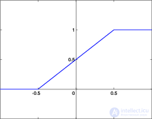
The signal at the output of the neuron is linearly related to the weighted sum of the signals at its input.
 ,
, Where  - function parameter. In artificial neural networks with a layered structure, neurons with transfer functions of this type, as a rule, constitute the input layer. In addition to a simple linear function, its modifications can be used. For example, a semilinear function (if its argument is less than zero, then it is zero, and in other cases, behaves as linear) or a step function (linear function with saturation), which can be expressed by the formula [10] :

In this case, the function can be shifted along both axes (as shown in the figure).
The disadvantages of the stepwise and semilinear activation functions relative to the linear one can be called the fact that they are not differentiable on the whole numerical axis, and therefore cannot be used when training with some algorithms.
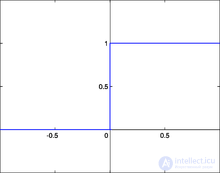
Another name is Heaviside function. It is a drop. Until the weighted signal at the input of the neuron reaches a certain level  - the output signal is zero. As soon as the signal at the input of the neuron exceeds the specified level, the output signal changes abruptly by one. The first representative of layered artificial neural networks - the perceptron [11] consisted exclusively of neurons of this type [5] . The mathematical notation for this function is as follows:

Here  - shift of the activation function relative to the horizontal axis, respectively
  it is necessary to understand the weighted sum of the signals at the inputs of the neuron without taking into account this term. Due to the fact that this function is not differentiable on the entire abscissa axis, it cannot be used in networks trained by the back-propagation error algorithm and other algorithms that require the differentiability of the transfer function.
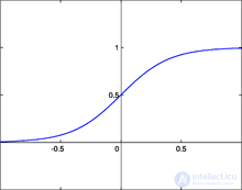
One of the most frequently used types of transfer functions at the moment. The introduction of sigmoid-type functions was due to the limitations of neural networks with a threshold neuron activation function — with such an activation function, any of the network outputs is either zero or one, which limits the use of networks not in classification tasks. The use of sigmoidal functions made it possible to switch from binary outputs of a neuron to analog ones [12] . Transmission functions of this type, as a rule, are inherent in neurons located in the inner layers of the neural network.
Mathematically, the logistic function function can be expressed as:

Here t is the parameter of the function that determines its steepness . When t tends to infinity, the function degenerates into a threshold one. With  sigmoid degenerates into a constant function with a value of 0.5. The range of values of this function is in the interval (0,1). An important advantage of this function is the simplicity of its derivative:

The fact that the derivative of this function can be expressed in terms of its value facilitates the use of this function when training a network using the backpropagation algorithm [13] . A feature of neurons with such a transfer characteristic is that they amplify strong signals substantially less than weak ones, since the areas of strong signals correspond to gentle characteristics. This prevents saturation from large signals [14] .
Using the hyperbolic tangent function

differs from the above logistic curve in that its range of values lies in the interval (-1; 1). Since the ratio is true
 ,
, then both graphs differ only in the scale of the axes. The derivative of the hyperbolic tangent, of course, is also expressed by a quadratic function of the value; the property of resisting saturation takes place just as well.
Using Modified Hyperbolic Tangent Function

scaled along the ordinate axis up to the interval [-1; 1] allows to obtain a family of sigmoidal functions.
The radial basis transfer function (RBF) takes as an argument the distance between the input vector and some pre-specified center of the activation function. The value of this function is the higher, the closer the input vector is to the center [15] . As a radial basis, you can, for example, use the Gauss function:
 .
. Here  - distance between the center
  and input vector
  . Scalar parameter
  determines the decay rate of the function when the vector is removed from the center and is called the window width , the parameter
  determines the shift of the activation function along the abscissa axis. Networks with neurons using such functions are called RBF networks. As a distance between vectors, various metrics can be used [16] , the Euclidean distance is usually used:
 .
. Here  -
-  -th component of the vector applied to the input of the neuron, and
  -
-  -th component of the vector determining the position of the center of the transfer function. Accordingly, networks with such neurons are called probabilistic and regression [17] .
In real networks, the activation function of these neurons may reflect the probability distribution of a random variable, or denote any heuristic dependencies between the quantities.
The functions listed above are only part of the set of transfer functions used at the moment. Other transfer functions include such as [18] :
 ;
;  ;
; The above described model of a deterministic artificial neuron, that is, the state at the output of the neuron is uniquely determined by the result of the work of the adder of input signals. Stochastic neurons are also considered, where neuron switching occurs with a probability depending on the induced local field, that is, the transfer function is defined as:
 ,
, where is the probability distribution  usually looks like sigmoid:
 ,
, a normalization constant  is introduced for the condition of normalizing the probability distribution
  . Thus, the neuron is activated with probability
  . Parameter
  - analogue of temperature (but not the temperature of the neuron) and determines the disorder in the neural network. If a
  direct to 0, the stochastic neuron will transition to a normal neuron with Heaviside's transfer function (threshold function).
A neuron with a threshold transfer function can simulate various logical functions. The images illustrate how it is possible, by setting the weights of the input signals and the sensitivity threshold, to force the neuron to perform a conjunction (logical “AND”) and a disjunction (logical “OR”) on the input signals, as well as a logical negation of the input signal [19] . These three operations are enough to simulate absolutely any logical function of any number of arguments.
|
Comments
To leave a comment
Models and research methods
Terms: Models and research methods