
Lecture
COMPUTING SYSTEM, - is a combination of hardware and software tools forming a unified environment intended for solving information-processing (computing) tasks. Initially, general-purpose computing systems were built on the basis of single-processor computers in order to increase their speed. In the earliest computers the processors themselves managed input/output operations. However, the speed of an external device is significantly lower than the speed of the processor, so during input/output operations the processor was effectively idle. To balance their operation, in the late 1950s – early 1960s computers began to be equipped with independent input/output processors for the parallel execution of computations and data-exchange operations, and it was then that the term “computing system” appeared. The main advantages of a computing system compared with a single-processor computer are: a significant increase in performance through static or dynamic parallelization of the process of solving a problem (e.g., executing separate parts of a task on different processors); an increase in the efficiency of equipment use through fuller loading of it; an increase in system reliability, and others.
A computing system (CS) is an interconnected combination of computer hardware and software intended for information processing.
Sometimes a CS is understood as the combination of a computer's technical means, which includes at least two processors linked by common control and by the use of system-wide resources (memory, peripheral devices, software, etc.).
The constant increase in the degree of integration and speed of the elements of modern microprocessors, their high level of reliability and relative cheapness make it possible to build computing systems by combining the required number of microprocessors and organizing parallel data processing. Parallelism in computation has considerably complicated the control of the computing process, as well as the distribution of hardware and software resources. For this reason an important role in a computing system has come to be assigned to the operating system, which performs the functions of scheduling the computing process and allocating resources (main and external memory, processors, peripheral equipment, etc.), as well as to optimizing compilers for high-level languages, which make it possible to make the fullest use of the architectural features of microprocessors. A major role in achieving high efficiency of a computing system's operation is played by the switching system that links the processors to one another or to the main-memory modules. As a rule, a common bus is used for this, to which the processors and memory modules are connected. In computing systems made up of several processors, matrix switches are typically used, as well as ring, star and other connection topologies. When a large number of processors are combined, more complex connection topologies are used – a torus, a hypercube, and others.
Modern computing systems differ greatly from one another in their capabilities and characteristics, and this accounts for the diversity of features by which computing systems are classified (e.g., by the types and number of computers or processors, system architecture, operating modes, methods of controlling the system's elements). Thus, computing systems may be separable (comprising several computers that are able to work independently of one another) and inseparable (or multiprocessor, consisting of processors, each of which can perform its functions only as part of the computing system). One type of inseparable computing system is clusters, consisting of several interconnected computers that are housed in a single enclosure or connected by a high-speed communication channel.
Computing systems are also divided into homogeneous and heterogeneous. A homogeneous computing system is built on the basis of processors or computers of a single type, while a heterogeneous one consists of computers or processors of different types. Multicomputer and multiprocessor computing systems are distinguished. In multicomputer computing systems each of the processors has its own local main memory and, as a rule, operates under the control of its own operating system, while in multiprocessor computing systems the processors work with shared main memory under the control of a single operating system. Classes of parallel computing systems are also distinguished: SMP (symmetric multiprocessing – a group of processors work with shared memory), MPP (massively parallel computing system – processors, whose number is practically unlimited, each work with their own memory), NUMA (an intermediate architecture combining properties of the SMP and MPP classes).
If, besides digital computers, a computing system also includes analog computers, it is classified as a hybrid computing system. These computing systems are usually used in modeling complex systems, dynamic processes, etc., for example in developing geological and technological models of oil and gas fields, or aircraft flight-control systems.
In 1966 M. Flynn (USA) proposed classifying computing systems by the number of instruction streams and data streams. He identified 4 classes: SISD (single instruction stream – single data stream), which includes systems with a single processor; SIMD (single instruction stream – multiple data streams), which includes homogeneous vector and matrix computing systems; MISD (multiple instruction streams – single data stream); MIMD (multiple instruction streams – multiple data streams), in which each processor operates on its own program and its own data. This classification remains relevant to this day, but it does not allow all types of computing systems to be characterized fully and precisely enough (e.g., dataflow systems), so attempts to more precisely systematize the whole variety of computing systems continue. For example, Basu's classification (USA, 1987) is based on the sequential determination of decisions adopted when designing a computing system: the level of parallelism (data, instructions or tasks), the method of implementing algorithms (hardware or software), the method of parallel instruction execution (pipelining or simultaneous independent execution), as well as the method of controlling the instruction-execution process (synchronous or asynchronous). Krishnamurthy (India, 1989) proposed classifying computing systems by four characteristics: the level of parallelism; the method of implementing parallelism (hardware or hardware-software), the topology (mesh, linear array, torus, tree, star, etc.), the degree of processor coupling (strong, weak, medium) and the mechanism of processor interaction (via message passing, shared variables or operand availability), and the method of control (synchronous, asynchronous, dataflow).
Important milestones in the development of computing systems were the creation of such systems as ILLIAC IV (put into service in 1974; a matrix computing system of 64 processors), the vector-pipeline “Cray-1” (1976, USA), “Cyber 205” (1981, USA), “Cray C90” (1991, USA), the massively parallel computing system “Connection Machine-1” (which combined 65,536 one-bit processors connected via a hypercube, 1985), “Cray T3E” (1995) and others. In Russia the computing systems PS-2000 (produced from 1981) and PS-3000 (produced in 1984–87) were manufactured, along with the multiprocessor computing complexes “Elbrus-1” (1980) and “Elbrus-2” (1985). The fastest computing system in Russia as of mid-2015 was “Lomonosov-2”, manufactured by the company “T-Platforms” and installed at Lomonosov Moscow State University. It occupies 31st place in the June edition of the international TOP500 supercomputer ranking, reaching a performance of 1.8 petaflops (1 petaflop = 10^15 floating-point operations per second) on the LINPACK benchmark, against a theoretical maximum of 2.6 petaflops for the equipment used. First place in TOP500, with a record performance of 33.8 petaflops, is held by the computing system “Tianhe-2”, designed by the National University of Defense Technology of the People's Liberation Army of China.
The resources of a computing system include those facilities of the computing system that can be allocated to a data-processing process for a given quantum of time. The main resources of a CS are processors, areas of main memory, data sets, peripheral devices, and programs.
A computing system with distributed memory – a system in which each processor has its own local memory, and there is no shared memory. The exchange of information between the components of the system is provided by means of a communication network through message passing.
Such systems often combine separate computers. This type of CS is called loosely coupled systems. Loosely coupled systems are found both in the SIMD class and in the MIMD class. This kind of CS construction removes the constraints inherent to a common bus, but leads to additional overhead for passing messages between processors or machines. The multiprocessor nature of a CS also gives rise to another problem – the problem of simultaneous access to memory by several processors.
Multiprogramming
Multiprogramming is a data-processing mode in which the resources of a computing system are provided to each process from a group of data-processing processes located in the CS, for intervals of time whose duration and order of allocation are determined by the control program of that system, with the aim of ensuring simultaneous operation in interactive mode.
Real-time mode
Real-time mode is a data-processing mode in which the interaction of a computing system with processes external to it is ensured at a rate commensurate with the speed at which those processes occur.
This data-processing mode is widely used in control systems and information-retrieval systems.
Single-program operating mode of a computing system (CS)
The hardware of a computer, together with its software, forms a CS. Depending on the class of computer and the type of operating system, a CS can operate in single-program and multiprogram modes.
In single-program mode, only one program resides and executes in the computer's memory at a time. This mode is typically characteristic of microcomputers and personal computers, that is, of computers for individual use.
Multiprogram (multiprogramming) operating mode of a computing system (CS)
In multiprogram (multiprogramming) operating mode, several programs reside in the computer's memory, and they are executed partially or fully between the processor's transitions from one task to another, depending on the situation arising in the system.
In multiprogram mode, machine time and main memory are used more efficiently, since when some situation arises in the task being executed that requires the processor to switch to a wait state, the processor switches to another task and executes it until a similar situation arises in that task, and so on.
When implementing multiprogram mode, it is necessary to determine the order of task switching and to choose the moments of switching so that the efficiency of use of machine time and memory is maximal.
Multiprogram mode is provided by the computer's hardware and by the operating system's facilities. It is characteristic of complex computers, where the cost of machine time is significantly higher than for microcomputers. Multiprogramming operating systems have also been developed that make it possible to simultaneously monitor the solution of several tasks and increase the efficiency of the user's work.
Batch-processing mode
Depending on the order in which user programs are executed in multiprogram mode, batch-processing mode and collective-access mode are distinguished.
In batch-processing mode, tasks are arranged in one or several queues and are selected for execution sequentially.
Collective-access mode
In collective-access mode, each user submits their task for execution at any moment in time, that is, for each user in such a CS an individual-use mode is implemented. This is usually accomplished by means of quantizing machine time, when each task residing in the computer's main memory is allocated a time quantum. After the time quantum ends, the processor switches to another task or continues executing the interrupted one, depending on the situation in the CS. Computing systems that provide users with collective access through the quantizing of machine time are called time-sharing CS.
A classification is defined by a set of features that characterize the internal parameters of the objects of classification. In doing so, the most important features are chosen, ones that determine the external parameters of these objects.
In the case where the objects of classification are computing systems (CS), the classification task is complicated by the diversity of CS application domains and, consequently, the diversity of CS types, since CS are specialized in accordance with the class of tasks being solved.
However, there are two factors that must be taken into account whatever types of CS are being considered. These are
The tasks to be solved can be divided, quite conditionally, according to the nature of interaction between the parts of the task (computing processes) into: tightly coupled and loosely coupled.
Let us call the computing facilities intended for solving the above-mentioned tasks, respectively:
The composition of computing facilities and the connections between these facilities are the main classification features that characterize any technical structure, including a CS, since a computing system is a technical structure.
Note that the CS considered here, according to M. J. Flynn's classification, belong to the group “multiple instructions, multiple data”.
As for the terms used below, among the possible synonyms preference is given, firstly, to Russian ones, where they exist (for example, multicomputer, rather than multicomputer-system), and secondly, to the simplest ones (for example, switch, rather than switching facilities or communication network). The recommended terms are further highlighted in italics.
A classification of CS by the main features characterizing the structure of these technical objects is given in Table 1. The table includes additional features reflecting the specifics of memory organization, data transfer, control, and design implementation of the CS.
Table 1 – Classification of CS
|
Classification feature |
|
|
|
Multiprocessor CS |
Multicomputer CS |
|
|
Structure composition |
CP*, PM, BM, EM, I/O, SW |
VM (computer, MPCS), EM, I/O, SW |
|
Type of connection between structural elements (type of switch) |
Matrix SW, multistage SW, common bus |
Bus-based (multibus SW and etc.) or link-based ( SW with regular connections and others ) |
|
Memory organization |
Shared memory |
Distributed memory |
|
Method of data transfer |
Parallel (strong coupling) |
Parallel-sequential (weak coupling) |
|
Receiver of transferred data |
– |
Cache memory or main memory |
|
Initiator of data transfer |
– |
Successor process or predecessor process |
|
Operating system (OS), control |
Shared,
centralized |
Copies of OS and common superstructure,
mixed |
|
Spatial placement of structural elements |
On a single board or in a single unit |
In a single unit, in a single rack, etc. (in a single room) |
* CP – central processor (does not contain SM cache memory); PM – processor module, i.e. CP+SM, where SM may be two-level; BM – main memory, which may consist of one or several MM modules (2, 4, 8 …);
MM – main memory module, which is sectioned memory with a number of sections equal to the number of words in an SM block (usually 4); EM – external memory on magnetic or optical storage media; I/O – input/output devices; SW – switch, i.e. the set of facilities that ensure interaction between structural elements. In addition to key elements, SW includes a control device that performs routing, arbitration, and similar functions; VM – computing module (this is a computer or an MPCS).
The image of a unified CS is supported by a combination of both hardware and software (the operating system). However, the classification given here is oriented mainly toward the organization of the hardware.
A diagram of the CS classification is given in Figure 1.
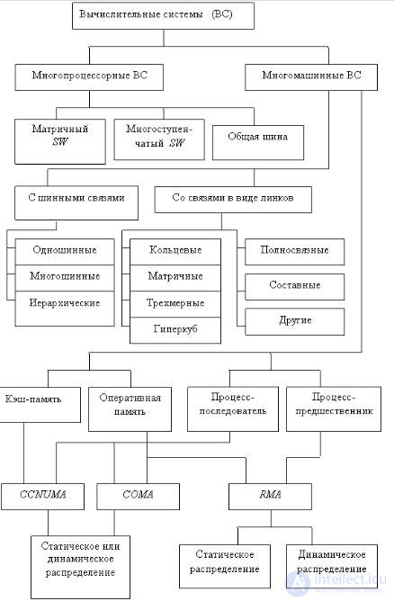
Figure 1 – Diagram of CS classification
Let us examine each type of CS in more detail.
Multiprocessor CS are characterized by strong coupling and shared memory.
A distinguishing feature of an MPCS is that the access time of any processor to memory is the same. In foreign literature such MPCS are called UMA (Uniform Memory Access) – CS with uniform memory access. The operation of an MPCS is also characterized by the abbreviation SMP (Symmetrical Multiprocessor Processing) – uniform (symmetric) multiprocessor processing, which is achieved through cyclic changing of processor priorities.
Multiprocessor CS with various switches are shown in Figure 2.

Figure 2 – Multiprocessor computing systems with different switches
a – MPCS with a crossbar switch; b – two-stage 16×4 switch;
c – MPCS with a common bus (the switch is “smeared” across RM).
Multicomputer systems (MCS) are characterized by weaker connections and distributed memory (figure 3).
Connections in an MCS may take the form of buses or links, i.e. two groups of lines along which signals can be transmitted independently in two opposite directions (figure 4).
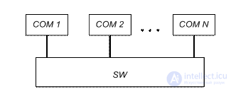
Figure 3 – A multicomputer system (MCS).
COM – computing node, SW – switch.
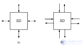
Figure 4 – A switching node (4 × 4) with connections in the form of buses (a) and in the form of links (b)
Figures 5–7 show MCS with bus connections.
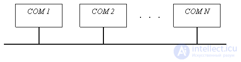
Figure 5 – An MCS with a common bus. COM – computing module
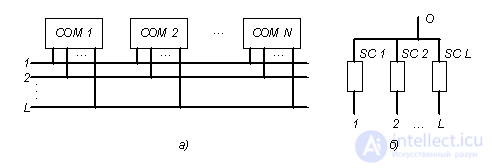
Figure 6 – Diagram of a multibus MCS (a) and the node of key elements included in each CM (b)
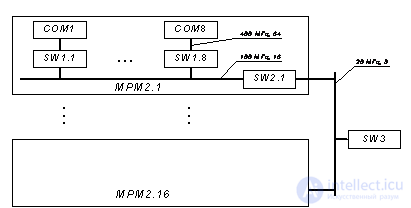
Figure 7 – An MCS with hierarchical bus connections.
COM – first-level computing module,
MRM – second-level computing module,
Some MCS with link-type connections can be called regular: ring, mesh (grid, torus, twisted torus), three-dimensional, hypercube. The switching nodes used to build such connections have a dedicated input/output for connecting to a CM and several links for connecting to neighboring nodes (figure 8).
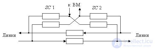
Figure 8 – A switching module for a regular ring-type MCS, , L = 2.
Variants exist with L = 4, 6, etc. SC – switching (key) elements
Figure 9 shows MCS in the form of a ring and a mesh (in the form of a torus).
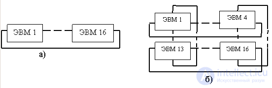
Figure 9 – Regular MCS in the form of a ring (a) and a torus (b)
The switching nodes used for fully connected and composite (including tree-structured) MCS have identical (link-type) inputs/outputs (figure 10). All connections are of the same type (links) and can be used both for connecting a CM and for connecting other switching nodes.
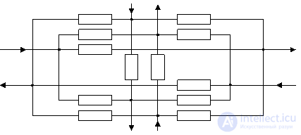
Figure 10 – A node of key elements 4×4 for composite MCS.
Variants exist with 8×8, 16×16, 22×22, 64×64, 128×128, etc.
Composite switching modules of 16×16, assembled from 4×4 switching nodes, are shown in figure 11. Figure 12 shows a 16×16 switching module assembled from 4×4 switching nodes.
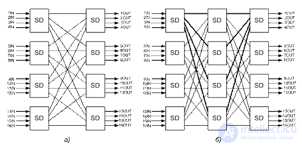
Figure 11 – A two-stage 16×16 switch built from 4×4 switching nodes. On the left – the input links, on the right – the corresponding output links. On the left, a blocking SW (a).
A non-blocking SW (b) can be obtained by adding another column of 4×4 switching nodes (a Clos switch)
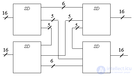
Figure 12 – A composite 64×64 switch made of 4 32×32 switching nodes.
Here each line is a pair of links (input and output)
Figure 13 shows a fully connected MCS with an N×N crossbar switch. For clarity of the figure, the input-link circuits of the computing nodes are not connected (points 1… N respectively). The switch can be implemented as shown in figures 11 (N = 16) or 12 (N = 64).
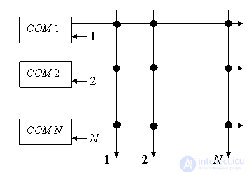
Figure 13 – An MCS with a crossbar switch
In all the MCS structures considered above, main memory is distributed across the CMs, and the access time of a processor to the main memory of “its own” CM is significantly less than the access time to the memory of “someone else’s” (remote) CM. In foreign literature such MCS are called NUMA (Non-Uniform Memory Access) – systems with non-uniform access to memory, and the memory itself – distributed (distributed memory).
Since the number of CMs in an MCS is usually large (≥64), the operation of an MCS is also characterized by the abbreviation MPP (Massively Parallel Processing) – a computing system with massively parallel processing.
By the method of organizing data transfer, i.e. the way a processor of one CM accesses the memory of another (remote, or “someone else’s”) CM, MCS can be divided into those organized as CCNUMA, COMA and RMA .
CCNUMA (Cache Coherent NUMA) – an MCS organization [architecture] in which a line of data is transferred on the initiative of the successor process. The data is transferred from the main memory of the CM in which it was obtained into the cache memory of the CM on which the successor process will run. The transfer takes place when the data is actually needed.
COMA (Cache Only Memory Architecture) – an MCS organization [architecture] in which a page of data is transferred on the initiative of the successor process. The data is transferred from the main memory of the CM in which it was obtained into the main memory of the CM on which the successor process will run. The transfer takes place when the data is actually needed. The memory of the CM is called attracting (AM – Attraction Memory), since the data, when needed, is as if attracted into this memory.
RMA (Reflector Memory Architecture) – an MCS organization [architecture] in which a page of data is transferred on the initiative of the predecessor process. The data is transferred from the main memory of the CM in which it was obtained into the main memory of those CMs on which the successor processes will run (in the case of static distribution), or into the main memory of all CMs (in the case of dynamic distribution of processes across processors). The memory of the CM is called reflecting (RM – Reflector Memory), since the data, once received, is mapped into the memories of the other CMs.
In 1966, at the Institute of Electronic Control Computers, under the direction of M. A. Kartsev, a preliminary design of the M-9 computing system was developed. Project team: E. V. Glivenko, V. A. Brik, L. Z. Liburkin, L. V. Ivanov, Yu. I. Galkin. In 1967, on the basis of a decision of the Commission of the Presidium of the Council of Ministers of the USSR and an order of the USSR Ministry of Instrument-Making, a preliminary technical design of the M-9 (“October”) was developed, carried out as part of the preliminary design of the “Aurora” system — a complex of radio-electronic equipment, including equipment for processing large flows of radar information.
The team behind the preliminary technical design of the M-9: M. A. Kartsev (chief designer), R. M. Akchurin, V. A. Brik, E. V. Glivenko, L. N. Kovalenko, V. P. Kuznetsova, L. Z. Liburkin, V. P. Filippov.
In the M-9 project, M. A. Kartsev laid down advanced ideas in the field of parallel information processing. Many of this project's solutions were inventions; many fruitful ideas have still not been implemented to this day. The designers of the M-9 were tasked with creating, using the component and technological base available at the level of the late 1960s to early 1970s, computing equipment with a performance of about 10^8-10^9 operations/s. The need for such equipment was faced by the developers of systems for observing artificial Earth satellites using radar stations (academician A. L. Mints and the team he led at the Radio Engineering Institute of the USSR Academy of Sciences). The computing equipment that existed in the country at that time provided a performance of about 10^5-10^6 operations/s.
Thus, as early as 1966–67, M. A. Kartsev was setting the task of raising the performance of computing systems by 2-3 orders of magnitude and outlining ways of solving this problem. He proposed a new architecture and structure for a computing system that could exploit the natural parallelism of the source information to be processed.
Presenting the M-9 project in 1967 at a symposium on computing systems and environments in Novosibirsk, M. A. Kartsev jokingly explained that “the M-220 machine is called that because it has a performance of 220 thousand operations/s, and the M-9 is called that because it provides a performance of 10^9 operations/s”.
The ideas of functional arithmetic for parallel computing, formulated in the M-9 project, were a generalization of the principles of vector and matrix processors. The M-9 architecture provided for the execution of arithmetic and logical operations on a new class of operands — not on numbers, but on functions of one or two variables, specified at discrete points. The functional-arithmetic instruction set provided for operators executed by a structure of multi-bit processors, in which a pair of functions specified in the input registers corresponded to a result function obtained in the output registers. Operators were also provided whose result was a number rather than a function. Operators of the second type dealt with functions written into the registers of a structure of single-bit processors. These functions, taking the values 0 or 1, served to select some subset from the information being processed (i.e. operators of characteristic functions of sets were introduced). Operators of the third type involved both functions and sets, which served as operands or results of execution. These operators served to transform a function on some set, or to obtain, as a result, some set related to a given function.
The structure of the M-9 computing system, proposed by M. A. Kartsev, consisted of several large blocks joined by powerful trunk connections. M. A. Kartsev called these blocks “bundles”.
The main computing power of the M-9 was to be provided by the “functional bundle” in the form of a “grid” of 32-by-32 processors performing operators on 16-bit operands. In each horizontal line of this matrix, which has 32 processors, additional shared arithmetic circuits were provided, allowing operations of the “sum of pairwise products” type (the dot product of vectors with 32 components each) to be performed in a single machine cycle. When multiplying two matrices, 32 elements of the resulting matrix could be obtained at once in a single cycle of the functional bundle's operation. The shared arithmetic circuits could perform summation with accumulation of the result, which made it possible, when necessary, to process vectors longer than 32 components. A “mask” in the form of a matrix of Boolean variables could be superimposed on the operators executed by the “grid” of processors of the functional bundle, which allowed execution of actions only by the elementary processors marked with ones in the mask.
Work with matrices of Boolean variables for the mask was to be performed by a special device made of 32-by-32 elementary single-bit computing units, called “picture arithmetic”. “Pictures” could not only be transformed, but also shifted along the coordinate axes. Arrays of Boolean variables on a “picture” could be expanded and contracted. Direct connections were provided between the processors of the functional “grid” and the processors of the picture arithmetic. This provided additional capabilities for controlling the computing process.
In addition to the functional bundle in the form of a “grid” of processors, convenient for solving two-dimensional problems, the M-9 project also provided for a functional line — a structure working with functions of one variable. This line, called the “numeric bundle”, consisted of 32 processors. These processors were to perform operators on a single function or on a pair of functions specified at 32 points, or operators on two functions or two pairs of functions specified at 16 points. That is, with a single operator code, the numeric bundle could perform one action (or 2, 4, 8 different actions) on pairs of operands 128 bits long (or 16, 32, 16 bits, respectively), including floating-point arithmetic calculations.
The vector operations of the numeric bundle were supplemented by “picture arithmetic” in the form of a line of 32 elementary Boolean-variable computing units — the “feature arithmetic”.
The M-9 also included an “associative bundle”, representing a line of elementary computing units performing comparison operators on operands (“greater than”, “less than”, “equal to”, “greater than or equal to”, etc.), as well as a unit for processing the resulting Boolean variables and masking the elementary computing units of this bundle. The associative bundle was intended for processing large arrays of input information by sorting it into subarrays by content. The operators of the associative bundle determined not a single number but vectors, each component of which was linked to one of the characteristics of the object described by that vector.
In terms of its principle of organizing parallel computation, the M-9 architecture can be classified as SIMD (a single instruction stream — multiple data streams). The multiprocessor functional arithmetic of each bundle was to work with shared main memory and permanent memory for storing programs.
Various combinations of the bundles described above (from 1 to 8) were meant to allow the M-9 to build multiprocessor computing systems with a performance ranging from 20 million operations/s to 1–2 billion operations/s. In particular, it was assumed that the M-10 would implement the numeric bundle, and the M-11 would contain 2 functional bundles, 1 associative bundle, 1 numeric bundle (M-10), and an external computing unit for interfacing with the controlled object.
Besides the transition from the traditional computer architecture, working with numbers, to a function-operator architecture, as discussed above, an additional gain in performance of 1–2 decimal orders of magnitude could be obtained through the second main idea proposed in the M-9 project. It consisted in the synchronous combining of several machines into a single computing system. With such synchronous combining, all the machines were to operate from a single clock generator, performing operations in 1–2 cycles. At the end of one operation and at the start of the next, an exchange was possible between any arithmetic and storage devices of the machines combined into the system.
The M-9 was a general-purpose computing system, substantially different from the universal computers (including multiprocessor ones) known at that time, and suitable for solving the most diverse classes of computational and logical problems, as well as control problems.
Such problems, requiring the performance of a supercomputer, arose in connection with the need to process large flows of information from measuring devices of major technological facilities, defense control facilities, and large-scale scientific experiments. Multiprocessor computing structures, such as the M-9, opened up possibilities for solving geometric problems, related, for example, to the automatic processing of images from bubble and spark chambers in nuclear physics, the processing of images obtained from artificial Earth satellites, and the processing and analysis of geological maps.
The M-9 project, rich in ideas that were new at the time, was not implemented in full, for a number of technical and organizational reasons. Above all, because of the level of component base and technology available in the late 1960s. M. A. Kartsev, at a meeting marking the 15th anniversary of the Scientific Research Institute of Computing Complexes (NIIVK) in 1982, said: “In 1967 we came forward with a rather bold project for the M-9 computing complex. This was in the year of the 50th anniversary of the October Revolution, so the computing complex was called “October”. For the USSR Ministry of Instrument-Making, where we were based at the time, this project turned out to be too much of a stretch (beyond the scope of that ministry's tasks). We were told: go to V. D. Kalmykov (Minister of the Radio Industry of the USSR), since you're working for him anyway. The M-9 project remained unrealized. But in 1969 development of the M-10 began, and its first prototype appeared in 1973. For a number of years this machine was the most powerful in the Soviet Union, and it continues to be produced and operated to this day. Unique scientific results were obtained on the M-10, especially in the field of physics”.
The numeric bundle of the M-9 project — the M-10 machine — was mass-produced from 1974 by the Zagorsk Electromechanical Plant. Its development was awarded the USSR State Prize in Science and Technology.
From the brief description of the M-9 project presented here, one can see that as early as the late 1960s M. A. Kartsev proposed fundamental innovations in the architecture of computers and computing systems: a RISC-type architecture with a reduced instruction set executed in 1 machine cycle, and a VLIW-type architecture with a long instruction word specifying operation codes for vectors of one length or another, executed simultaneously in two or more multiprocessor arithmetic units.
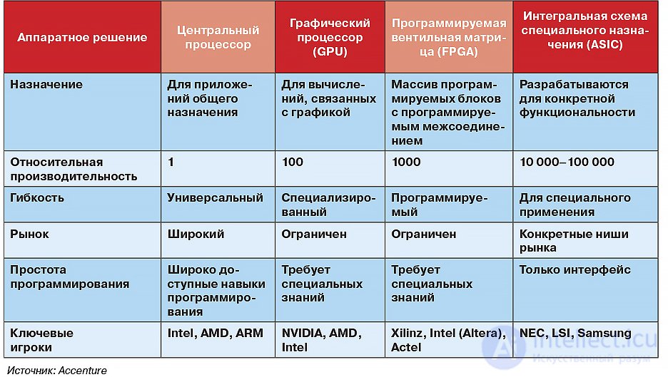
Heterogeneous computing systems — electronic systems that use different types of computing units. The computing units of such a system can be a general-purpose processor (GPP), a special-purpose processor (for example, a digital signal processor (DSP) or a graphics processing unit (GPU)), a coprocessor, or acceleration logic (an application-specific integrated circuit (ASIC) or a field-programmable gate array (FPGA)).
In general, a heterogeneous computing platform contains processors with different instruction set architectures (ISA). The demand for increased heterogeneity in computing systems is partly related to the need for high-performance, highly responsive systems that interact with other environments (audio/video systems, control systems, network applications, etc.).
The CPU is responsible for handling logical transactions and sequential computation, while the GPU focuses on performing parallel-processing tasks with a large number of threads (large-scale computation tasks).
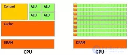
(Comparison of the original network, CPU and GPU architectures)
To put it more popularly, a processor is like a pen — you can use it to draw anything you want. A graphics processor is like a printer, and printing is certainly faster, but it requires interaction from the central processor.
Heterogeneous computing platforms have become the new favorites, and among heterogeneous computing there are also powerful forces, of which there are three different types.
The CPU + GPU type, the CPU + FPGA type, and the CPU + ASIC type.
In the past, technological advances and frequency scaling allowed most computer applications to increase performance without structural changes or hardware acceleration. Although these advances continue, their impact on modern application software is not as significant as the impact of certain obstacles, such as the memory wall[en] and the power wall
Now, with these additional constraints, the main method for obtaining additional performance from computing systems is the introduction of additional specialized resources, as a result of which the computing system becomes heterogeneous. This allows the developer to use several types of computing elements, each of which is capable of performing the tasks it is best suited for.
Adding additional, independent computing resources inevitably means that most heterogeneous systems are regarded as parallel computing systems or multicore systems.
Another term sometimes used for this type of computing is “hybrid computing” . Hybrid-core computing[en] — a form of heterogeneous computing in which asymmetric computing devices coexist within a single processor.
High-performance computing systems (HPC) — are applications and workloads involving the execution of resource-intensive computing operations using various resources.
Specialized high-performance computing solutions help organizations make discoveries that transform their business. High-performance computing has become more accessible than ever before, both on individual local systems and in clusters, including in the cloud.
Scientists, engineers and researchers use high-performance computing systems to perform incredibly resource-intensive tasks, including weather forecasting, oil and gas exploration, physics research, quantum mechanics research, and so on.
Although high-performance computing can be performed on a single system, truly powerful capabilities open up when using clusters of multiple high-performance computing nodes, which are also called supercomputers. They open up possibilities for large-scale modeling that would be impractical or even impossible to carry out on standalone systems.
Many of the first and most famous supercomputers were developed by Cray, which today is a partner of the Intel® Datacenter Builders program. Modern supercomputers are large clusters of nodes that include processors, accelerators, high-performance communication infrastructure, and comprehensive memory and storage systems. All these resources are available to different nodes, which helps prevent bottlenecks and ensure optimal performance.
Vertical scaling of performance
High-performance computing applications leverage the capabilities of hardware and software architectures that distribute computation among the resources of a single system (typically a server). This form of parallel processing is called vertical scaling. The performance gain is very significant, but it is limited by the capabilities of a single system.
Horizontal scaling of performance
High-performance computing applications can also distribute computing tasks across different systems configured to work together as a complex. Such a complex is called a high-performance computing cluster and allows applications to distribute computing tasks for parallel execution across multiple systems.
High-performance computing systems are increasingly used by organizations. They are also becoming more accessible. Scientists and engineers can run high-performance computing workloads on local infrastructure, as well as scale computing power without significant capital investment by using resources from cloud service providers.
Examples of use of high-performance computing systems
Modern enterprises use high-performance computing systems for simulation and modeling in many important areas, including the development of autonomous driving models, product design and manufacturing, analysis of seismic waves and their impact on structures, evaluation of oil and gas extraction strategies, and so on. High-performance computing systems are also useful for advancing precision medicine, financial risk assessment, fraud detection, fluid dynamics calculations, and so on.
Components of high-performance computing systems
The most effective high-performance computing systems are built on an ideally matched combination of hardware and software. The hardware typically includes high-performance processors, communication infrastructure, memory, storage resources, network components, and accelerators for special workloads. Platform software, libraries, optimized big-data and deep-learning infrastructures, and other software tools for high-performance computing systems help extract the greatest return from high-performance computing clusters.
Intel Corporation offers a full range of hardware and software for high-performance computing systems. These are high-performance computing systems based on Intel technologies.
At the core of everything are Intel® Xeon® Scalable processors, enabling the creation of revolutionary high-performance computing systems with record levels of flexibility and scalability. They are complemented by Intel® solutions for Ethernet networks and the Intel® Omni-Path Fabric (Intel® OP Fabric) infrastructure for optimizing scaling. Intel® Optane™ DC technologies deliver innovation in memory and storage, while Intel® FPGAs provide acceleration for specific workloads. Intel® software and developer tools help make the most effective use of the capabilities of Intel® architecture and technologies.
Intel Corporation offers a wide range of products and technologies for high-performance computing systems of various scales. Intel Corporation helps implement computing solutions that operate on exabytes of data for work on the most complex scientific problems, and offers a standards-based approach to solutions for the most common high-performance computing tasks, implemented in the Intel® HPC Platform Specification. High-performance computing systems are becoming increasingly accessible, and Intel Corporation helps users realize the benefits of new high-performance computing technologies.
Convergence of high-performance computing systems and artificial intelligence
Combining the capabilities of high-performance computing systems with machine- and deep-learning solutions offers enormous potential in fields ranging from linguistics to genomic sequencing and modeling of the global climate. Intel Corporation supports the convergence of high-performance computing systems and artificial intelligence by collaborating with ecosystem partners on the creation of reference architectures and solutions oriented toward practical application in specific domains.
Recent advances in computing technology and software are driving the development of high-performance computing systems. Intel Corporation will continue to work with enterprises in the high-performance computing ecosystem to optimize hardware performance, combine the capabilities of high-performance computing, AI and analytics, and select the optimal transition plan for workloads that use exabytes of data.
For high-performance computing systems, quantity matters, because computations can run in parallel across many nodes of a cluster.

Comments