Lecture
Let us consider an approximate model of a symmetrical vibrator.
The symmetrical vibrator is the simplest and at the same time the most widespread resonant device among antennas. It serves as the initial element for many of their types, as well as a model for assessing their gain. Therefore, before moving on to the characteristics and operating principle of antennas, it is necessary to familiarize yourself with the theory of the symmetrical vibrator ( dipole ).
A dipole antenna , or dipole , is the simplest and most popular class of antennas. It consists of two identical conductors, wires, or rods, usually with bilateral symmetry. Transmitters are supplied with current, and receivers receive a signal between the two halves of the antenna. Both sides of the feeder at the transmitter or receiver are connected to one of the conductors. Dipoles are resonant antennas, that is, their elements serve as resonators in which standing waves pass from one end to the other. So the length of the dipole elements is determined by the length of the radio wave.
The term "dipole" is translated as "two-pole" and means that the half-wave emitter is cut in its geometric center. The resulting two "poles", or power terminals, are connected to the feeder from the transmitter or receiver (see Fig. 6.1).
Any extended conductor of electric current, be it a wire, a rod or a tube, is characterized by quite specific values of inductance and capacitance, uniformly distributed along its length. This is explained by Fig. 6.2, a, which shows inductances L1 - L7 with their capacitances and capacitances C1 - C4, distributed between sections of the conductor.

Fig. 6.1 - Model of a symmetrical vibrator with power supply
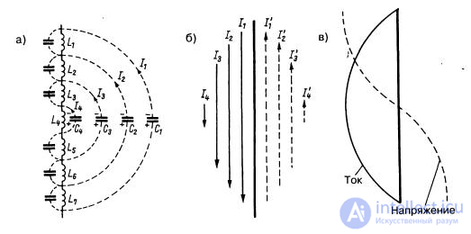
Fig. 6.2 — Current distribution in a half-wave conductor
Let all the capacities be charged at a certain moment, that is, acquire potential. Following
then they will begin to discharge through their inductances, resulting in a current and the emergence of a corresponding magnetic field.
When the capacitor C4 is discharged, current I4 will flow through the inductance L4;
SZ will be discharged through L3, L4 and L5 when current Ι3 flows;
discharge of C2 through L2 - L6 will cause current I2.
Finally, C1 will discharge through L1 - L7 at current I1.
It follows that the greatest current, equal to the sum of the currents in the range I1 - I4, will flow in the middle part of the emitter;
the current will decrease towards its ends, where it will turn to zero.
For greater clarity, the currents I1 - I4 are shown in Fig. 6.2, b in a different form. Under the action of current, magnetic fields are formed around the inductors.
They will again impart charges of opposite polarity to the capacitors, so the sign of the voltage will change.
Now the process will be repeated, but in the direction opposite to that shown in Fig. 6.2, with the help of currents I1 - I4. With all the simplifications, the picture shown in Fig. 6.2 gives an idea of the resonant distribution of current and
voltage in a half-wave radiator.
The voltage and current are shifted in phase by 90°, while the phase difference of the voltages at the ends of the emitter is 180°.
If we refine all the approximations, then we will use the equations of a long line of length l and transfer the reference system to
connection point of the input terminals. Then the system of equations will look like:
From the distribution of current and voltage in a half-wave emitter it follows that in its middle part the current is maximum (current antinode),
and the voltage is zero (voltage node). At the ends of the emitter the relationships are opposite: the voltage antinode coincides with the current node.
It is also clear from the voltage distribution that the half-wave elements can be attached in the geometric center with a conductive bracket directly to the grounded antenna support, since the attachment at the zero voltage point does not require insulation.
Therefore, it is permissible to ground half-wave elements in the geometric center. But then the voltage in the middle of the emitter turns out to be somewhat different from zero. The same happens with the current at the ends of the emitter, where it does not reach zero due to the end effect.
So it would be more correct to talk about current and voltage minima.
As can be seen from Fig. 6.2, c, the current is always maximum in the middle part of the half-wave vibrator, which is in a state of self-resonance.
The current decreases sinusoidally towards the ends of the vibrator, where it becomes zero. The maximum voltage is observed here,
sinusoidally decreasing towards the middle of the vibrator. There it becomes so small that in the first approximation it can be taken as equal to zero.
Strictly speaking, the voltages and currents are distributed across the vibrator not quite sinusoidally.
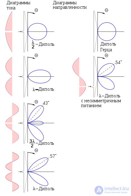
Let's look at some examples. Hertz dipole,
The current distribution is as shown in Fig. 6.3.
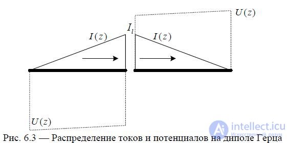
Half-wave vibrator when 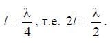 .
.
The current distribution is as shown in Fig. 6.4.
Fig. 6.4 — Distribution of currents and potentials on a half-wave vibrator
The currents on both arms are in phase, which is favorable from the point of view of forming directional radiation.
Wave vibrator when 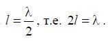 .
.
The current distribution is as shown in Fig. 6.5.
Fig. 6.5 — Distribution of currents and potentials on a wave vibrator
The wave vibrator works like two half-wave vibrators.
Symmetrical vibrator with arm length
The current distribution is as shown in Fig. 6.6.
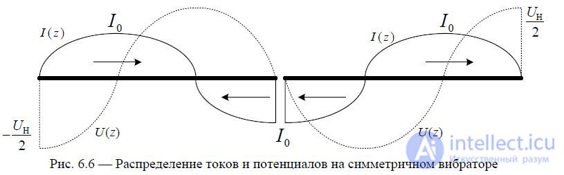
With  any symmetrical vibrator, antiphase current sections appear,
2 which have an adverse effect on the radiation characteristics when the radiation intensity in the direction of the main maximum decreases.
In this case, the emitted power is redistributed in lateral directions.
Symmetrical vibrator with arm length l = λ . The current distribution has the form shown in Fig. 6.7.
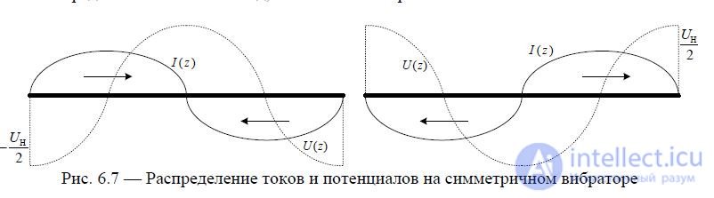
Fig. 6.7 — Distribution of currents and potentials on a symmetrical vibrator
Since the in-phase and out-of-phase currents are equal, there is no radiation in the main direction.
A rigorous solution to the current distribution problem shows that the current at the nodes is somewhat different from zero. This is due to the fact that the vibrator, unlike the two-wire line, radiates.
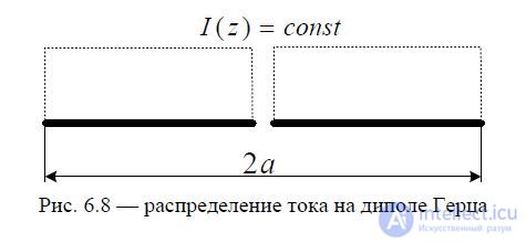
Let us consider the Hertz dipole and the current distribution on it (see Fig. 6.8).
To analyze the radiation field of antennas, several main radiation zones are distinguished.
The induction zone or near zone (Fresnel zone) of an elementary radiator is a region of space where in the expressions for E and H the terms proportional to 1/r^2 and 1/r^3 predominate over the terms proportional to 1/r. The radiated electromagnetic field in the Fresnel zone has a vortex character.
The radiation zone (Fraunhofer zone), wave zone or far zone of an elementary radiator is a region of space in which the terms proportional to 1/r are predominant. The radiated electromagnetic field in the far zone is a spherical wave in which the electric and magnetic vectors are perpendicular to the direction of propagation, i.e. it is a transverse electromagnetic wave.
Let us consider a vertical Hertzian dipole located in a Cartesian coordinate system (see Fig. 6.9).
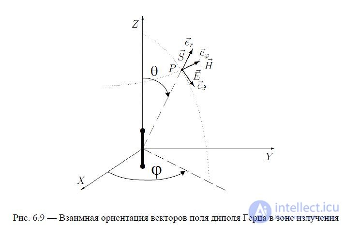
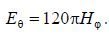
Figure 6.9 shows the mutual orientation of the field vectors of the Hertz electric dipole in the radiation zone. It should be noted that for the Hertz dipole, the electric field strength vector at any point (observation point) in the radiation zone is directed along the tangent to the circle lying in the plane passing through the observation point and the dipole axis. In particular, in the example considered (the dipole axis coincides with the OZ axis of the spherical coordinate system), the vector E at any point in the radiation zone is directed along the unit vector eϑ, and the vector H is directed along the unit vector eϕ, as shown in Figure 6.9.
The electric dipole field is characterized by three components: 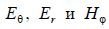 , of which the longitudinal component Er can be neglected, since it is proportional
The components of the field  are related by the relation
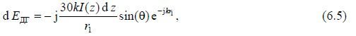
Thus, it is sufficient to investigate only one E component of the Hertz dipole radiation field. We will omit the index in what follows  . The electric transverse component of the dipole field is determined by the expression
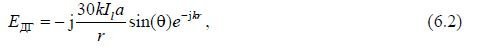
where r is the distance to the observation point located in the far zone. The amplitude of the electric dipole field is determined by the expression
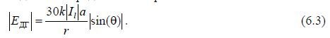
The amplitude  does not depend on the angle
  , i.e. This is stated on the website https://intellect.icu . The radiation field of the Hertz dipole has EDH axial symmetry.
When  there is no radiation, i.e. the dipole does not radiate in the axial direction.
When  the maximum radiation field is observed, the direction is orthogonal to the 2nd axis of the dipole - the main direction.
Determination of the radiation pattern.
The directivity pattern (DP) of a transmitting antenna over a field is a graphical representation of the dependence of the modulus of the complex amplitude of the intensity vector of the electric component of the electromagnetic field created by the antenna in the far zone on the angular coordinates θ and φ of the observation point in the horizontal and vertical planes, that is, the dependence E(θ,φ).
It is customary to denote the DN by the function f(θ,φ). The DN is normalized - all values of E(θ,φ) are divided by the maximum value Emax and the normalized DN is denoted by the function F(θ,φ).
Any antenna has a certain directivity, described by the corresponding diagram. To accurately display the directivity, it is necessary to construct its three-dimensional (spatial) image. But the spatial distribution of density is difficult to depict graphically, so it is usually enough to present the antenna's directivity diagram in the vertical and horizontal planes (in the main sections).
The antenna radiation pattern can be depicted in a polar coordinate system or in a section of this system, as well as in Cartesian (rectangular) coordinates.
Polar coordinates use a grid of concentric circles and rays emanating from their center (Fig. 6.10). Concentric circles represent stress, and at their center it is equal to zero.
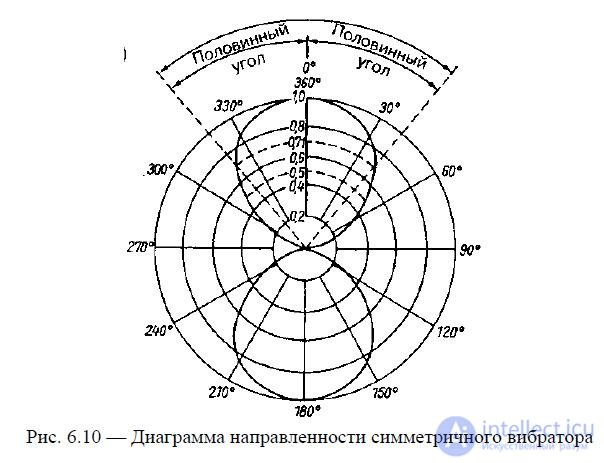
Fig. 6.10 - Directional diagram of a symmetrical vibrator
Fig. 6.10 shows the normalized radiation pattern of a half-wave vibrator in the horizontal direction.
plane (plane E, the beam width of the DN along the field, determined at a level of 0.707 from the maximum, is 80°).
The radiation pattern is used to determine a number of important parameters of the antenna under consideration. Half the width of the main lobe is called the half-level angle. This is the angle between the direction of maximum radiation and the direction where the energy flux density is half of the maximum. To determine this angle, the point of greatest voltage in the main direction is assigned a value of 1.0 and points are found on both sides of the radiation lobe where the voltage is 0.707 of the maximum. A decrease in voltage by a factor of 0.707 corresponds to a decrease in power by 50% or 3 dB. Then, as shown in Fig. 6.10, straight lines are drawn from the center through these points, which serve as the sides of the sought half-level angle. Usually, it is preferable to use the concept of the half-power pattern width or the 3 dB width. The half-power pattern lobe width is equal to the sum of both half-level angles and denotes the range of angles in which the energy flux density is not less than half of its maximum value.
The point of the radiation pattern where the voltage decreases to zero is called the zero point. Its position is described by the angle of the zero value, i.e. the angle between the direction of maximum radiation and the direction to the first zero point. The width at the zero level is the interval of angles between the first zero points on both sides of the main lobe of the radiation pattern.
The radiation pattern is normalized when all voltage values are divided by its maximum value and the result of the division is expressed as a fraction of a unit or as a percentage.
To describe the position of the planes in which the directional diagrams are constructed, the concepts of the E plane and the H plane are used. The first of these corresponds to the direction of the electric field lines in a plane wave front, the second to the direction of the magnetic field lines (see Fig. 6.9).
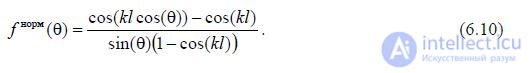
According to (6.3), the radiation pattern of the Hertz dipole is described by the function
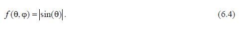
In the E-plane, the DN constructed according to (7.3) has the form shown in Fig. 6.11 — in blue.
Since for the Hertz dipole  does not depend on
  , then in the H-plane the radiation pattern has the form shown in Fig. 6.11 in red - the radiation pattern is circular.
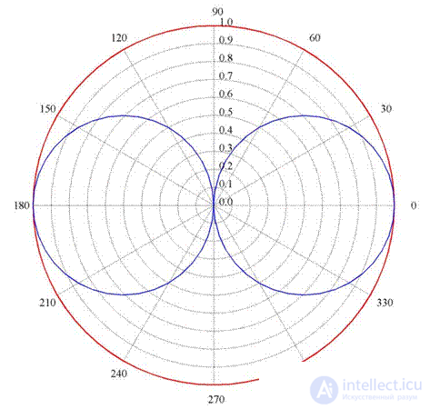
Fig. 6.11 — Directional patterns of the Hertzian dipole in the main sections
The radiation patterns obtained in Fig. 6.11 allow us to reconstruct the three-dimensional RP of the dipole.
Hertz, which has the form shown in the section in Fig. 6.12.
Fig. 6.12 — Section of the three-dimensional DP of the Hertzian dipole
Dipoles are non-directional antennas. Because of this, they are often used in communication systems.
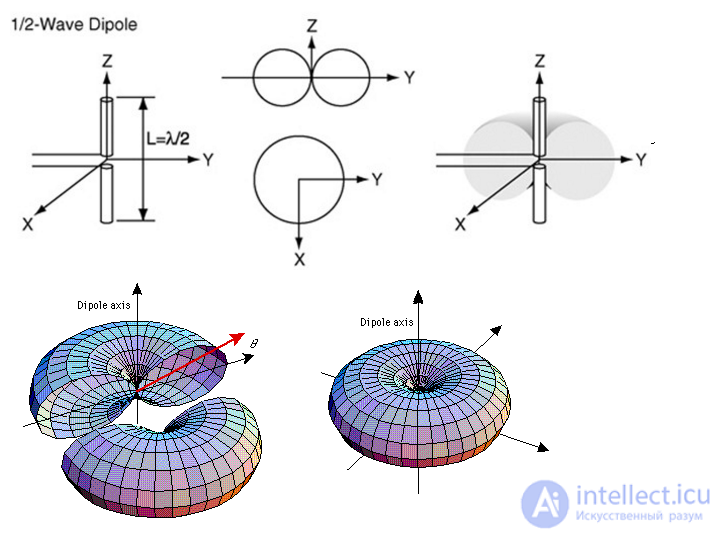
Fig. Directional diagram of a dipole antenna
Depending on the ratio of the vibrator length to the wavelength and the location of the feeder connection, its directional pattern takes the form shown in the figure:
The power radiation pattern can be found if the radiation intensity of the field at the receiving location is known, which is determined by the value of the Poynting vector.
Thus, the power radiation pattern  is determined from the field radiation pattern
  based on the relationship
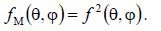
In the Cartesian coordinate system, the Hertzian dipole radiation patterns for field and power have the form shown in Fig. 6.13.
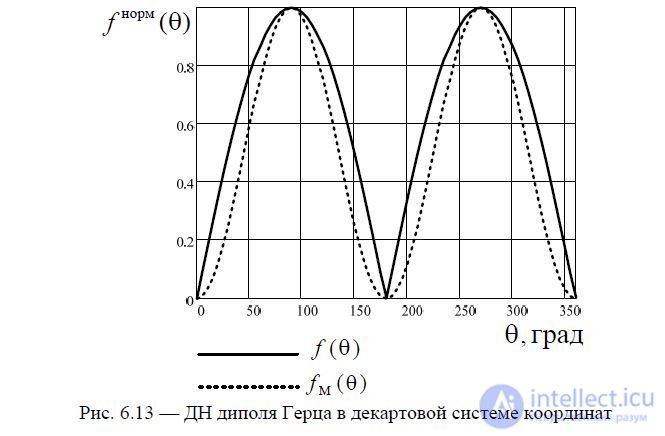
Fig. 6.13 — Hertzian dipole radiation pattern in the Cartesian coordinate system
Let us mentally divide the vibrator into an infinitely large number of elements dz. Since the length of each element is infinitely small, we can assume that within its limits the current does not change either in amplitude or in phase. Thus, the entire vibrator can be considered as a set of elementary electric vibrators dz and, accordingly, the field of the vibrator under consideration can be represented as the result of the addition (interference) of the fields radiated by the elementary vibrators. In view of the smallness of the air gap (gap) between the arms of the vibrator, we can neglect the influence of the electric field (magnetic current) existing in it on the radiation, and assume that the electric current flows along a solid conductor of length 2l.
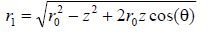
We select an element of length dz on the vibrator at point z and determine the field created by this element at an arbitrary observation point M, located at a distance r0 from the center of the vibrator (in the radiation zone for all elementary vibrators) at an angle  to its axis (Fig. 6.14).
Fig. 6.14 - Towards the determination of the radiation field of a symmetrical vibrator
Due to the small size of the element, it can be assumed that the current in it is constant along its length and has a complex amplitude I(z). In this case, the distance from the element to the point M is r1. The element under consideration can be considered an elementary radiator - a Hertz dipole, therefore, the field created by it, according to (6.3), will be determined by the expression
where I(z) is the complex current on the elementary emitter. Let us find the value of r1. As can be seen from Fig. 6.5,
We will use the well-known approximate expression 1+ x ≈1+ x/2 – x2/8, which is true for x < 1. Taking the value r0 out from under the root in (6.5) and leaving the terms containing z to a power not exceeding 2, we obtain
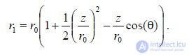
If point M is sufficiently far from the vibrator, then all rays connecting the antenna points with point M are practically parallel. Let us drop a perpendicular from point z in Fig. 6.14 in the direction r0 . As a result, for r1 we obtain the relation

Thus, we can define the far zone of the antenna as a region of space for each point of which all rays coming from the antenna to this point are parallel. The quantity r z cos() is often called the path difference of rays coming from the center of the vibrator and from the point with coordinate z. Since the observation point is at a large distance from
vibrator, then the value of Δr is small compared to r0 and the distances r0 and r1 differ little from each other. Based on (6.6), we obtain an expression for the phase factor in (6.5)
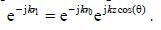
After transformation (6.5) we obtain the expression

The final expression for the radiation field of a symmetrical vibrator

In r0 sin() As in the case of the Hertz dipole, formula (6.7) consists of three factors: a factor that determines only the magnitude of the field strength and does not depend on the direction of
60I0
given point A factor that determines the directional properties (directivity characteristic r0)
and the phase factor je jkr . From (6.8) it is evident that the symmetrical vibrator has directional properties only in the E plane, and these properties are determined only by the ratio of the length of the vibrator arm to the wavelength l/λ.
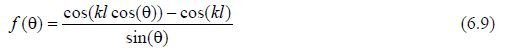
We will conduct the analysis of the symmetrical vibrator pattern based on formula (6.8).
From (6.9) it is evident that a symmetrical vibrator has directional properties only in the E plane, and these properties are determined only by the ratio of the length of the vibrator arm to the wavelength l/λ.
Along the axis (in the direction  ) the wire with current does not radiate. Let's consider several cases:
- Hertz dipole, when
- symmetrical vibrator with shoulder length
The results of calculations of the radiation patterns in the E-plane using formula (6.9) are presented in Fig. 6.15.
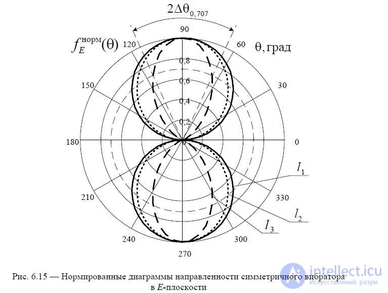
The beam width is determined as shown in Fig. 6.15.
If the length of the arm of a symmetrical vibrator  is , then in the direction,
perpendicular to the axis of the vibrator, i.e. in the equatorial plane  the fields of all elementary emitters are in phase, and, consequently, the field in this direction is maximum.
Increasing the length of the vibrator to a value  is accompanied by an increase
radiation in the direction perpendicular to the vibrator axis (the main radiation direction) due to the reduction of radiation in other directions. In this case, the DP becomes narrower (Fig. 6.15).
Let's consider a few more cases: symmetrical vibrators with arm lengths  .
.
The calculation results are presented in Fig. 6.16.
With increasing ,  the directivity characteristic passes through 0 not only at
  , but also at some other values of this angle. The main lobes become narrower, but side lobes appear, radiation in the main direction
decreases. The decrease in radiation in the main direction is explained by the following: the resulting phase shift of the fields radiated by elementary emitters in a given direction is determined by the spatial phase shift and the phase shift of the currents of these elementary emitters.
When  sections with antiphase currents appear on the vibrator, the length of which increases as the ratio increases
  .
.
Therefore, in this case, although in the main direction the spatial phase shifts are equal to zero, the fields radiated by the out-of-phase currents of the elementary emitters are added out-of-phase.
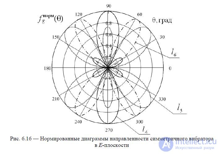
Fig. 6.16 - Normalized radiation patterns of a symmetrical vibrator in the E -plane
The growth of the ratio  is also accompanied by the growth of the side lobes, and when
  the field strength in the direction of the maximum of the side lobe becomes equal to the field strength in the main direction, and with further increase
  exceeds it.
At  (or at
  , where n is an integer) there is no radiation in the main direction, since the antiphase sections of the vibrator have the same length.
In practice, symmetrical vibrators are used, in which  the maximum radiation coincides with the main direction.
In the future we will consider exactly such vibrators. The normalized directional diagram of such
vibrator, is described by the expression
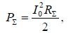
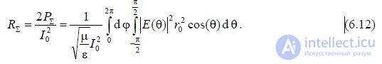
The power  emitted by a symmetrical vibrator can be found using the Poynting vector method, i.e. by integrating the average value of the Poynting vector over the surface of a sphere of large radius (in the far zone), at the center of which the vibrator is located. Just as in the case of a Hertzian dipole, we can write
where  is the radiation resistance, referred to the current in the antinode l
With the length of the arm,  the radiation resistance is recalculated to the input terminals of the antenna using the formula
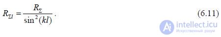
In general, the radiation resistance related to the current antinode is determined by the formula
Substituting the expression for the directivity characteristic (6.8) into (6.12) (without phase factors), we obtain
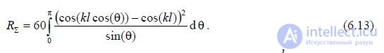
As can be seen from (6.13), the value  depends only on the ratio
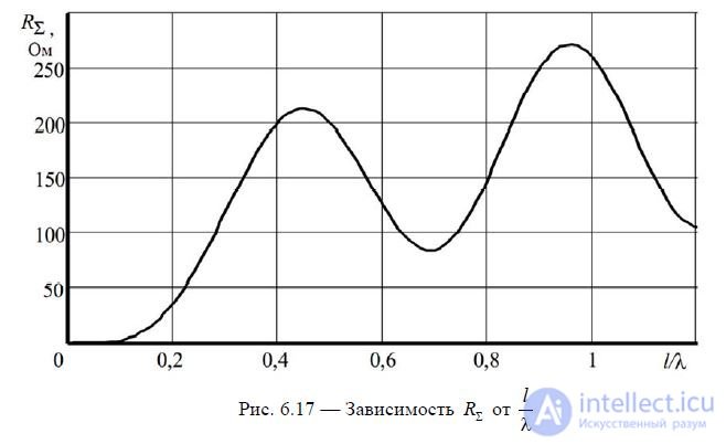
  . This formula is approximate, since it is derived for a sinusoidal distribution of current over the vibrator, which is only true for very thin vibrators. However, the results of calculations using (6.13) agree well with the experimental data. This is explained by the fact that the radiation resistance is determined by the field in the far zone, which depends little on the thickness of the vibrator. Figure 6.17 shows the graph of the dependence of calculated using (6.13)
  on
on  .
.
The oscillating nature of the dependence is explained by the fact that the interference pattern of the field in the far zone changes with a change in the ratio  .
.
Next, we will determine the input resistance of a symmetrical vibrator. The power radiated by the vibrator (or any antenna) corresponds to the active radiation resistance. The power loss corresponds to the active loss resistance. Along with the radiated electromagnetic field, there is an electromagnetic field oscillating near the antenna and associated with it, which corresponds to reactive power. The latter corresponds to the reactive resistance of the antenna.
Thus, the generator connected to the antenna is loaded with a complex impedance, called the input impedance of the antenna. The input impedance of a symmetrical vibrator (as well as other wire antennas) is equal to the ratio of the voltage at the vibrator terminals (feed points) to the current at the feed points
In what follows we will omit the loss resistance. For a symmetrical vibrator with l 0.25, we can use the approximate equivalent circuit of the emitter,
based on the introduction into the model of a long line of radiation resistance, referred to the input terminals - see Fig. 6.18.
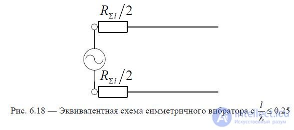
For an open transmission line, its input resistance is determined by  and taking into account the radiation resistance included in the line, the input resistance of a symmetrical vibrator
  can be approximately calculated using the formula

where 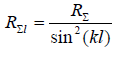 , and
, and  is determined from the graph in Fig. 6.17.
For a symmetrical vibrator with,  one can use an approximate equivalent circuit of the emitter, based on the introduction into the model of a long line of radiation resistance, connected at the current antinode point, which is located at a distance from the ends of the emitter arms - see Fig. 6.19, a.
Knowing the property of an open line segment of length, we can move on to the equivalent
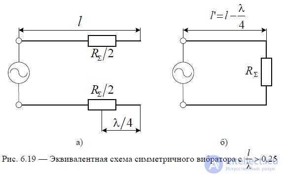
4 the symmetrical vibrator circuit shown in Fig. 6.19, b. Then the input resistance of the symmetrical vibrator can be determined by the formula
where the wave impedance of a symmetrical vibrator is determined by the formula 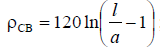 ;
;
a — radius of the conductor;
the value of the coefficient of traveling waves is determined by the formula KBV =  (at
(at  );
);
line segment
Based on (6.15), we will calculate the input impedance of the symmetrical vibrator as a function of  . See Fig. 6.20, which shows graphs for the active (6.20, a) and reactive (6.20, b) components of the input impedance for different values of the symmetrical vibrator's wave impedance
  . It is clear that with decreasing
  dependence R ВХ and X вх are smoothed out. This is essential for matching the antenna with the feeder line. We will calculate the VSWR dependencies corresponding to the graphs of the antenna's input impedance shown in Fig. 6.20. The calculation results are shown in Fig. 6.21. It is clear from the figure that with decreasing wave impedance of the symmetrical vibrator,
  the matching band expands.
antennas with a feed line. This property of a symmetrical vibrator is widely used in practice. A reduction  can be achieved by increasing the width of the conductors that form the arms of the symmetrical vibrator.
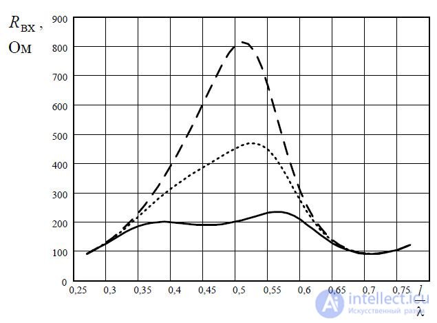
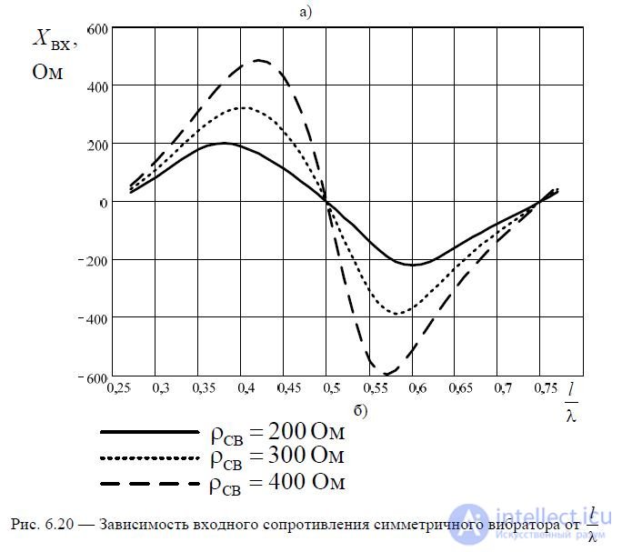
Fig. 6.20 — Dependence of the input resistance of a symmetrical vibrator on
Fig. 6.21 — Dependence of the SWR at the input of a symmetrical vibrator on
Effective length of the antenna. In the case of vibrator antennas, it is sometimes convenient to use a calculation parameter called the effective length of the antenna. The effective length of  a symmetrical vibrator (or other antenna) is called the length
an imaginary vibrator with a uniform current distribution 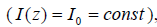 creating in the direction of maximum radiation (at
  ) a field equal to the field of a given antenna in the direction of its maximum radiation. In this case, the currents at the feed points of both antennas are considered equal.
Based on the condition of equality of the current moments, we determine the effective length of a symmetrical vibrator
After transformations we obtain an expression for determining the effective length l D
Taking into account (6.16), we can write an expression for the normalized radiation pattern of a symmetrical vibrator based on (8.4) in the form
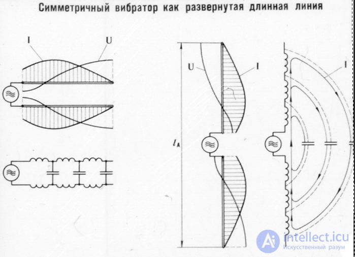
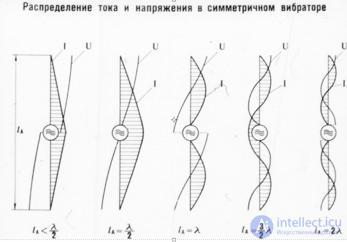
Current and voltage distribution in a symmetrical vibrator
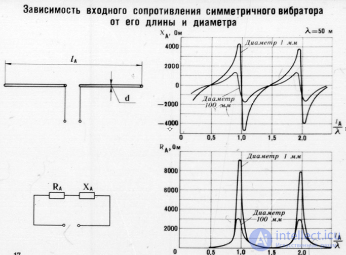
dependence of the input resistance of a symmetrical vibrator on its length and diameter
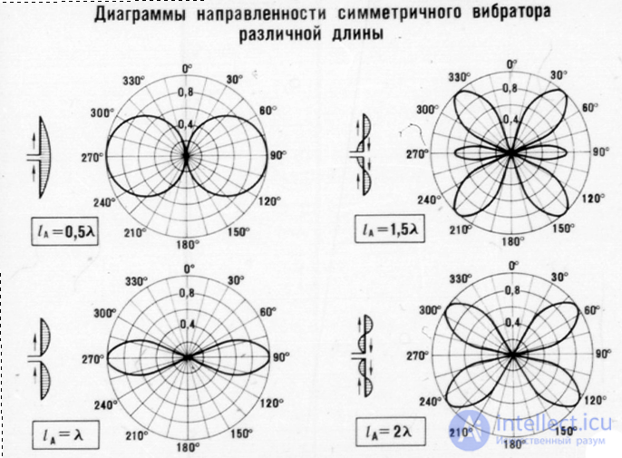
Directional patterns of a symmetrical vibrator depending on its length
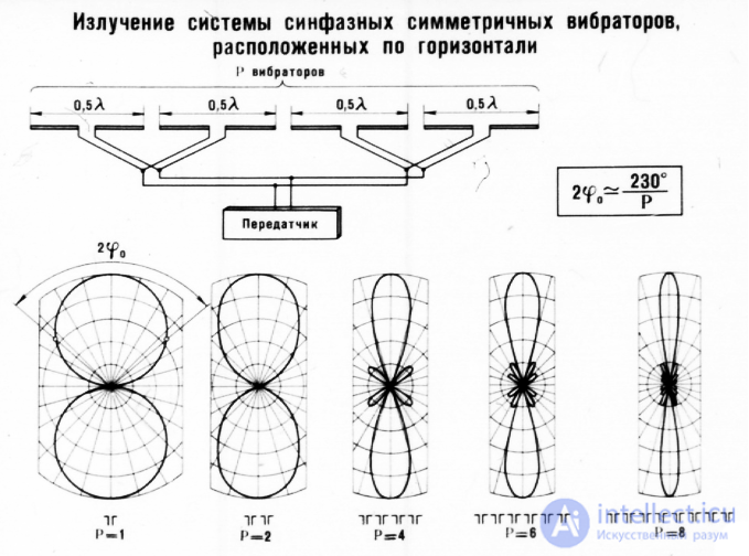
Radiation of a system of in-phase symmetrical vibrators located horizontally
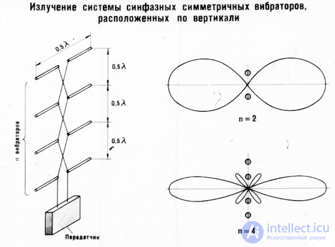
Radiation of a system of in-phase symmetrical vibrators located vertically
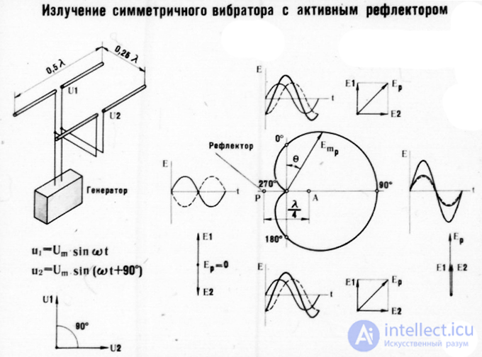
Radiation of a symmetrical vibrator with an active reflector
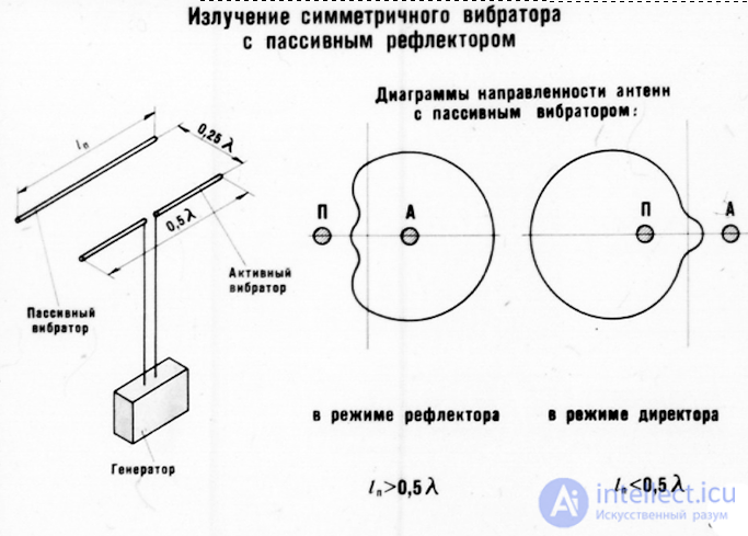
Radiation of a symmetrical vibrator with a passive reflector
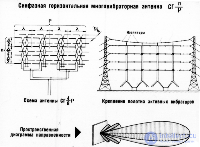
in-phase horizontal multivibrator antenna

Comments