
Lecture
Suffix structures are structures for representing the suffixes of strings; examples of such structures are the suffix tree and the suffix array. They are used in algorithms for substring search, determining the similarity of strings, and others.
Let us examine these structures in more detail.
Suffix tree — a trie containing all the suffixes of some string (and only them). It lets us determine whether the string w occurs in the original string t in time O(|w|), where |w| is the length of the string w.
 is a nonempty finite set of symbols called the alphabet. A sequence of symbols (possibly empty) from the alphabet is denoted by the letters r, s, and t.
 represents the reversed string. Individual symbols are denoted by the letters x, y, or z.
  is the empty string. The symbols of the alphabet are the letters a, b, …. For now the size of the alphabet is assumed to be constant. |t| denotes the length of the string t.
  is the set of all strings of length m,
  and
and 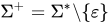 .
.
Prefix w of a string t is a string such that wv = t for some (possibly empty) string v. A prefix is called proper if |v|  0.
0.
Suffix w of a string t is a string such that vw = t for some (possibly empty) string v. A suffix is called proper if |v| 0. For example, for the string «substring» the substring «sub» is a proper prefix, and «ring» is a proper suffix.
The substring w of the string t is called a right extension if t can be represented as  and
and  for some strings
  and
and  , as well as letters x y. A left extension is defined analogously. For example, for «eabceeabcd» the substring «abc» is a right extension, since in both its occurrences in t it is followed by different symbols, whereas the same substring is not a left extension, because in both occurrences it is preceded by the same symbol «e».
 -tree T is a rooted tree with edges labeled by sequences from . For each symbol a of the alphabet, every node in the tree T has at most one edge whose label begins with the symbol a. The edge from t to s labeled v we will denote by
  .
.
Let k be a node of the -tree T; then path(k) is the string that is the concatenation of all the edge labels from the root to k. We call  the location of w, for which path() = w.
Since each branch is unique, if path(t) = w, we can denote the node t by . The subtree of the node is denoted by .
.
The words represented in the -tree T are given by a set denoted by words(T). A word w belongs to the set words(T) if and only if there exists a string v (possibly empty) such that  is a node of the tree T.
If the string w belongs to words(T), w = uv,  is a node of the tree T, the pair
  we will call a reference pair w with respect to the tree T. If u is the longest prefix such that is a reference pair, we will call the canonical reference pair. Then we will write
  . The location is called explicit if |v| = 0, and implicit otherwise.
-tree T, in which every edge is labeled by a single symbol, is called atomic (for it, every location is explicit). -tree T, in which every node is either the root, a leaf, or a branching node, is called compact.
An atomic -tree is also called  (a ray). Atomic and compact -trees are uniquely determined by the words they contain.
Suffix tree for a string t is a -tree such that words(T) = {w| w is a substring of t}. For a string t, the atomic suffix tree is denoted ast(t), and the compact suffix tree is denoted cst(t).
Reverse prefix tree of a string t is the suffix tree for the string .
Embedded suffix is a suffix that occurs in the string t somewhere else as well. The longest embedded suffix is called the active suffix of the string t.
Lemma. The location w is explicit in the compact suffix tree if and only if w is a non-embedded suffix of t, or w is a right extension.
Proof.  . If is explicit, then it can be either a leaf, a branching node, or the root (in that case
  and w is an embedded suffix of t).
If is a leaf, then it is also a suffix of t. Hence it must be a non-embedded suffix, since otherwise it would occur somewhere else in the string t:  v is a suffix of t such that w is a prefix of v. This node cannot be a leaf.
If is a branching node, then there must exist at least two outgoing edges from with different labels. This means there exist two distinct suffixes u, v, such that w is a prefix of u and w is a prefix of v, where v = wxs, u =  , x
, x  . Therefore, w is a right extension.
 . If w is a non-embedded suffix of t, it must be a leaf. If w is a right extension, then there are two suffixes u and v, u = wxs, v = , x , then w is a branching node. The lemma is proved.
Now it is easy to see why the answer to the question of whether the word w occurs in the string t can be found in time O(|w|): one need only check whether w is a location (explicit or implicit) in cst(t).
The edge labels must be pointers to positions in the string, so that the suffix tree uses O(n) memory. The label (p, q) of an edge denotes the substring  or the empty string if p > q.
Ukkonen introduces the term open edges for edges that end in leaves. The labels of open edges are written as (p,  ) instead of (p, |t|), where is a length always greater than |t|.
Let T be a -tree. Let  be a node of T, v the longest suffix of w such that
  is also a node of T. The unlabeled edge from to is called a suffix link. If v = w, it is called atomic.
Claim. In ast(t) and cst(t$), where $  t, all suffix links are atomic.
Proof. The symbol $ is called the sentinel symbol. The first part (for ast(t)) follows from the definition, since the locations are explicit. To prove the second part (the case of cst(t)), we must show that for every node is also a node of cst(t). If is a node of cst(t), then it is either a leaf or a branching node. If it is a leaf, then aw is a non-embedded suffix of t. Thanks to the sentinel symbol, it follows from the lemma that all suffixes (including the root, the empty suffix) are explicit, since only the root is an embedded suffix. Therefore w is a leaf or the root. If is a branching node, then aw is a right extension, and so is w. Consequently, the location is explicit by the lemma. The claim is proved.
As follows from this proof, the sentinel symbol guarantees the existence of leaves for all suffixes. With such a symbol there can be no embedded suffixes except the empty one. If we omit the sentinel symbol, some suffixes may become embedded, and their locations will become implicit.
Claim. A compact suffix tree can be represented in a form requiring O(n) memory.
Proof. A suffix tree contains at most one leaf per suffix (exactly one with the sentinel symbol). Every internal node must be a branching node, hence an internal node has at least two children. Each branching increases the number of leaves by at least one, so we have at most n internal nodes and at most n leaves.
To represent the strings that serve as edge labels, we use indexing into the original string, as described above. Each node has at most one parent, and thus the total number of edges does not exceed 2n.
Similarly, each node has at most one suffix link, so the total number of suffix links is also bounded by 2n. The claim is proved.
As an example of a suffix tree with 2n-1 vertices, consider the tree for the word  . The size of the atomic suffix tree for a string t is O(
 ).
).
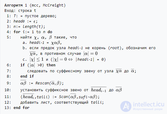
The mcc algorithm begins with an empty tree and adds suffixes starting with the longest one. The mcc algorithm is not an on-line algorithm, that is, it requires the entire string to be available in order to run. For correct operation, the string must end with a special symbol, different from all others, so that no suffix is a prefix of another suffix. Each suffix in the tree will correspond to a leaf. For the algorithm we define is the current suffix (at step
  ),
),  (head) is the longest prefix of the suffix that is also a prefix of another suffix
  , where
  .
.  (tail) we define as
 .
.
The key idea of the mcc algorithm is the relationship between and  .
.
Lemma. If where
where  is a letter of the alphabet,
  is a string (possibly empty), then is a prefix of .
Proof. Let . Then there exists , , such that
  is a prefix both of
  and of
  . Then is a prefix of and , hence, is a prefix of the head . The lemma is proved.
We know the location , and if we have a suffix link, we can quickly move to the location — the prefix of the head — without needing to find the path from the root of the tree. But the location } might not be explicit (if the location  was not explicit at the previous step), and the suffix link might not yet be established for the node. The solution given by McCreight finds the node
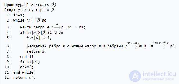
  in two steps: «rescanning» and «scanning». We walk up the tree from the node until we find a suffix link, follow it, and then apply rescanning of the path to the location (which is simple, because we know the length and this location exists, so we do not need to read the full edge labels while moving down the tree — we can simply check only the initial letters and the lengths of the words).
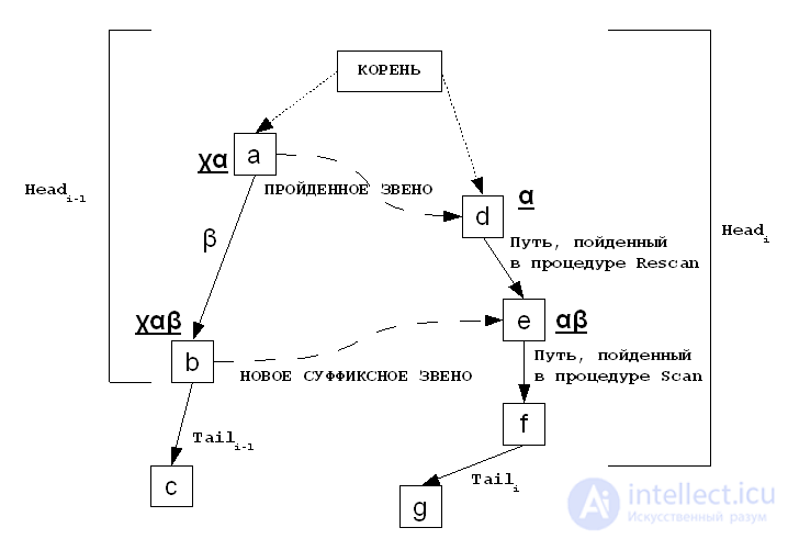
The figure illustrates this idea. Instead of trying to find the path from the root to the node  , the algorithm moves to , follows the suffix link to
  , performs a rescan of the path to the (possibly implicit) location
  , and it remains to find the path to , walking character by character.
The algorithm consists of three parts.
1. First it determines the structure of the previous head, finds the next available suffix link, and follows it.
2. Then it rescans the part of the previous head whose length is known (this part is called  ).
).
3. Finally the algorithm sets the suffix link for , scans the remaining part of (called ), and adds a new leaf for .
A branching node is created in the second phase, the rescanning phase, if the location does not exist. In this case scanning is not necessary, because if were longer than  , then
  would be a right extension, but by the lemma } is also a right extension, so the node
  must already exist. The node is created in the third phase if the location is still not explicit.
Note that if  then
then  is also found just as quickly, as when following the suffix link according to line 7 of the algorithm.
The Rescan procedure searches for the location . If the location is not yet explicit, a new node is added. This happens when the head (  ) has been scanned completely: if the head is longer (and the node is already defined), } must be a prefix of more than two suffixes and is also a left extension
  . The location can only be explicit if this node is already a branching node, and if was not a left extension then must have been longer, because a longer prefix was encountered.
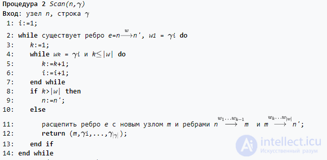
The Scan procedure performs a depth search of the tree and returns a position.
The algorithm invented by Esko Ukkonen for building a suffix tree in linear time is probably the simplest of such algorithms. This simplicity comes from the fact that the algorithm can first be presented as a simple but inefficient method, which, through several "common-sense" implementation techniques, reaches the level of the best algorithms in terms of worst-case running time.
For Ukkonen's algorithm we will need
1) Implicit suffix trees
2) General description of the algorithm
3) Optimizing the algorithm
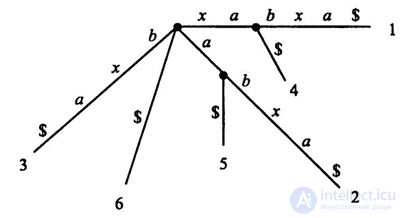
Suffix tree for the string xabxa$
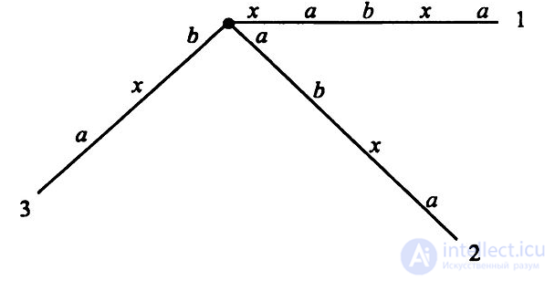
Implicit suffix tree for the string xabxa$
Ukkonen's algorithm builds a sequence of implicit suffix trees, the last of which is transformed into the actual suffix tree of the string S.
The implicit suffix tree of the string S is the tree obtained from the suffix tree of S$ by removing all occurrences of the terminal symbol $ from the edge labels of the tree, then removing edges left without labels, and then removing vertices that have fewer than two children. The implicit suffix tree of the prefix S[l..i] of the string S is obtained similarly from the suffix tree for S[l..i]$ by removing the $ symbols, edges, and vertices, as described above.
The implicit suffix tree for any string S will have fewer leaves than the suffix tree for the string S$ if and only if at least one of the suffixes of S is a prefix of another suffix. The terminal symbol $ was added to the end of S precisely to avoid this situation. This is a very important point in the definition of an actual suffix tree. However, if S ends with a symbol that does not appear anywhere else in S, then the implicit suffix tree for S will have a leaf for every suffix and will therefore be an actual suffix tree.
Although an implicit suffix tree may not have leaves for all suffixes, all the suffixes of S are encoded in it — each is spelled out by the symbols along some path from the root of this implicit suffix tree. However, if this path does not end in a leaf, there will be no marker indicating the end of the path. Thus implicit suffix trees are themselves somewhat less informative than actual ones. We will use them only as an auxiliary tool in Ukkonen's algorithm to obtain the actual suffix tree for S.
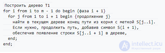
Ukkonen's algorithm builds an implicit suffix tree Ti for every prefix S[l..i] of the string S, starting with T1 and increasing i by one until Tm has been built. The actual suffix tree for S is obtained from Tm, and the entire process requires time O(m). We will explain Ukkonen's algorithm by first presenting a simple method by which all the trees are built in time O(m³), and then we will optimize the implementation of this method so that the stated speed is achieved.
To turn this general description into an algorithm, we must specify precisely how to perform a suffix extension. Let S[j..i] = β be a suffix of S[1..i]. In extension j, when the algorithm finds the end of β in the current tree, it extends β to ensure the presence of the suffix βS(i + 1) in the tree. The algorithm follows one of the following three rules.
Rule 1. In the current tree the path β ends at a leaf. This means that the path from the root labeled β reaches the end of some «leaf» edge (an edge leading into a leaf). When updating the tree, the symbol S(i + 1) must be appended to the end of the label of this leaf edge.
Rule 2. No path from the end of the string β begins with the symbol S(i + 1), but there is at least one path beginning from there. In this case a new leaf edge must be created, starting at the end of β, labeled with the symbol S(i + 1). Here, if β ends inside an edge, a new vertex must be created. The leaf at the end of the new leaf edge is assigned the number j. Thus, rule 2 has two possible cases.
Rule 3. Some path from the end of the string β begins with the symbol S(i + 1). In this case the string βS(i + 1) is already present in the current tree, so nothing needs to be done (in an implicit suffix tree, the end of a suffix does not need to be marked explicitly).
Suffix array is a lexicographically sorted array of all the suffixes of a string. This data structure was developed by Gene Myers and Udi Manber as a more memory-efficient alternative to the suffix tree. It is often used where fast substring search is needed, for example in the Burrows–Wheeler transform (BWT), and also as a data structure in a search index.
Given a string  of length
  .
.
The  -th suffix of the string is the substring
  ,
,  .
.
Then the suffix array of the string  is the permutation of suffix indices
  ,
,  , which specifies the order of the suffixes in lexicographically sorted order. In other words, we need to sort all the suffixes of the given string.
For example, for the string  the suffix array will be:

In 1989, Manber and Myers published a paper in which they described the suffix array data structure and how to use it for substring search. Suffix array is an array of the lexicographically sorted suffixes of a string (if this terminology is unfamiliar, you can look at the «problem statement» section of that paper). Generally speaking, there is no point in storing the suffixes themselves — it is enough to store the starting position of each suffix — but defining the array this way is easier to understand. Here is an example for the string «mississippi»:
Consider the string «abracadabra», 11 characters long.

Sorted list of its suffixes:
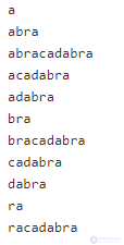
The suffix array of this string is {11,8,1,4,6,9,2,5,7,10,3}, because the suffix «a» starts at the 11th character, the suffix «abra» starts at the 8th, and so on, up to the last suffix «racadabra», which starts at the third character of the original word.
Now, using this array, we can easily find all substrings. For example, if we need to find the substring «ab», it is enough to find all the suffixes that begin with «ab». Because of the alphabetical sort, they are located next to each other. Using binary search, we find the 2nd and 3rd suffixes «abra» and «abracadabra», which correspond to the 2nd and 3rd elements of the suffix array (8 and 1). This means that the sought substring «ab» occurs at the first and eighth characters of the original word.
The algorithm described above sorts the cyclic shifts (if a dollar sign is not appended to the string), and therefore  will give the sought position of the smallest cyclic shift. The running time is
  .
.
Suppose that in the text  we need to search for the string in online mode (i.e., the string must be considered unknown in advance). We build the suffix array for the text in
  . Now we will search for the substring as follows: note that the sought occurrence must be a prefix of some suffix . Since the suffixes are ordered for us (this is what the suffix array gives us), the substring can be searched for using binary search over the suffixes of the string. The comparison of the current suffix and the substring inside the binary search can be done trivially, in
  . Then the asymptotic complexity of the substring search in the text becomes
  .
.
Given a string , after performing some preprocessing on it, we need to be able to answer, in  , queries comparing two arbitrary substrings (i.e., checking whether the first substring is equal to/less than/greater than the second).
We build the suffix array in  , while keeping the intermediate results: we will need the arrays
  from every phase. Therefore the memory required will also be .
Using this information, we can, in , compare any two substrings whose length is a power of two: for this it is enough to compare the equivalence-class numbers from the corresponding phase. Now we need to generalize this method to substrings of arbitrary length.
Suppose now a new query arrives to compare two substrings of length  starting at indices and
  . We find the largest block length that fits inside a substring of that length, i.e., the largest
  such that
  . Then comparing the two substrings can be replaced by comparing two pairs of overlapping blocks of length
  : first we compare the two blocks starting at positions and , and if they are equal — compare the two blocks ending at positions
  and
and  :
:


Thus, the implementation turns out to be roughly as follows (here it is assumed that the calling procedure itself computes , since doing this in constant time is not so easy (apparently the fastest way is precomputation), but in any case this has nothing to do with the application of the suffix array):
Given a string , after performing some preprocessing on it, we need to be able to answer, in  , queries for the longest common prefix (longest common prefix, lcp) of two arbitrary suffixes at positions and .
The method described here requires of extra memory; another method, using a linear amount of memory but a non-constant query time, is described in the next section.
We build the suffix array in , while keeping the intermediate results: we will need the arrays from every phase. Therefore the memory required will also be .
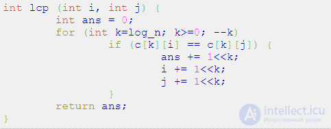
Suppose now a new query arrives: a pair of indices and . We use the fact that we can, in , compare any two substrings whose length is a power of two. To do this, we iterate over the powers of two (from larger to smaller), and for the current power check: if the substrings of that length match, we add this power of two to the answer, and continue looking for the longest common prefix to the right of the matching part, i.e., we must add the current power of two to and .
Implementation:
Here  denotes the constant equal to the base-2 logarithm of , rounded down.
Given a string , after performing some preprocessing on it, we need to be able to answer queries for the longest common prefix (longest common prefix, lcp) of two arbitrary suffixes at positions and .
Unlike the previous method, the one described here will perform preprocessing of the string in time using  memory. The result of this preprocessing will be an array (which is itself an important source of information about the string, and can therefore be used to solve other problems). Answers to a query will then be produced as the result of an RMQ query (range minimum query) on this array, so depending on the implementation one can achieve either logarithmic or constant running time.
The basis for this algorithm is the following idea: let us find, in some way, the longest common prefixes for each pair of suffixes adjacent in sorted order. In other words, let us build an array  , where
  equals the longest common prefix of the suffixes
  and
and  . This array will give us the answer for any two adjacent suffixes of the string. Then the answer for any two suffixes, not necessarily adjacent, can be obtained from this array. Indeed, suppose a query arrives with some suffix numbers and . Let us find these indices in the suffix array, i.e., let
  and
and  be their positions in the array
  (let us order them, i.e., let
  ). Then the answer to this query will be the minimum in the array
  , taken over the segment
  . Indeed, the transition from suffix to suffix can be replaced by an entire chain of transitions, starting with the suffix and ending at the suffix , but including all the intermediate suffixes lying between them in sorted order.
Thus, if we have such an array , then the answer to any longest-common-prefix query reduces to a range minimum query on the array . This classical range minimum query problem (RMQ) has many solutions with different asymptotics, described here.
So, our main task is the construction of this array . We will build it alongside the algorithm for building the suffix array: at each current iteration we will build the array for cyclic substrings of the current length.
After the zeroth iteration, the array obviously must be zero.
Suppose now we have completed the  -th iteration, obtained from it the array
  , and must, on the current -th iteration, recompute this array, obtaining its new value . As we recall, in the suffix-array construction algorithm, cyclic substrings of length were split in half into two substrings of length
  ; let us use this same trick for building the array .
So, suppose that on the current iteration the suffix-array construction algorithm has done its work and found the new permutation value of the substrings. Let us now walk through this array and look at pairs of adjacent substrings: and ,  . Splitting each substring in half, we get two different situations: 1) the first halves of the substrings at positions and differ, and 2) the first halves coincide (recall that such a comparison can easily be made by simply comparing the class numbers from the previous iteration). Let us consider each of these cases separately.
1) The first halves of the substrings differ. Note that in this case, at the previous step these first halves must have been adjacent. Indeed, equivalence classes cannot disappear (they can only appear), so all distinct substrings of length will give (as first halves) distinct substrings of length at the current iteration, and in the same order. Thus, to determine in this case, we simply need to take the corresponding value from the array .
2) The first halves coincide. Then the second halves could either coincide or differ; moreover, if they differ, they need not have been adjacent at all on the previous iteration. Therefore, in this case there is no simple way to determine . To determine it, we must proceed in the same way as we plan to later compute the longest common prefix for any two suffixes: we must perform a minimum query (RMQ) on the corresponding segment of the array .
Let us estimate the asymptotic complexity of this algorithm. As we saw when analyzing these two cases, only the second case increases the number of equivalence classes. In other words, we can say that each new equivalence class appears together with one RMQ query. Since the total number of equivalence classes can be up to , we must also search for the minimum with asymptotic complexity  . For this, we need to use some data structure for range minimum queries; this data structure will need to be rebuilt from scratch on every iteration (of which there are a total of ). A good choice of data structure would be a segment tree: it can be built in , and then queries can be performed in , which gives us exactly the overall asymptotic complexity .
Implementation:
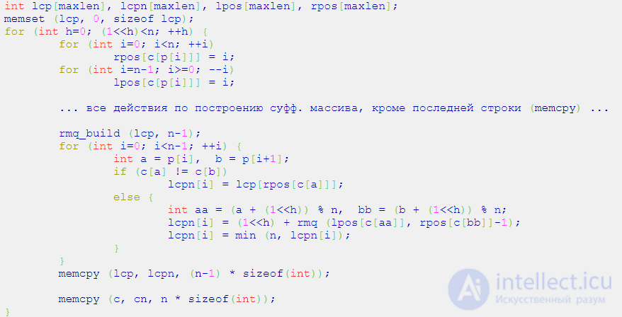
Here, besides the array  , a temporary array
  is introduced holding its new value. We also maintain the array
  , which for each substring stores its position in the permutation . The function
  is some function that builds a data structure for range minimum over the array given as the first argument, with its size passed as the second argument. The function
  returns the minimum over a segment: from the first argument to the second, inclusive.
From the suffix-array construction algorithm itself we only had to factor out the copying of the array , since during the computation of we will need the old values of this array.
It's worth noting that our implementation finds the length of the common prefix for cyclic substrings, whereas in practice the length of the common prefix for suffixes in the usual sense is more often needed. In this case, one simply needs to cap the values of after the algorithm finishes:
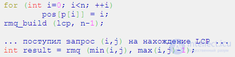
For any two suffixes, the length of their longest common prefix can now be found as the minimum over the corresponding segment of the array :
Let us perform the preprocessing described in the previous section: in time and memory, we find, for each pair of suffixes adjacent in sorted order, the length of their longest common prefix. Now let us use this information to find the number of distinct substrings in the string.
To do this, we will look at which new substrings start at position , then at position  , and so on. In effect, we take the next suffix in sorted order and look at which of its prefixes give new substrings. In this way we obviously will not miss any of the substrings.
Using the fact that our suffixes are already sorted, it is not hard to see that the current suffix will give, as new substrings, all of its prefixes except those coinciding with the prefixes of the suffix  . That is, all of its prefixes except the first
  will give new substrings. Since the length of the current suffix equals
  , we finally obtain that the current suffix gives
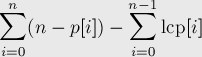
  new substrings. Summing this over all suffixes (for the very first one, , there is nothing to subtract — we simply add
  ), we obtain the answer to the problem:



Comments