
Lecture
come in the following types
2-3 tree
B-tree
Fusion tree
Rope
Splay tree
Tango tree
AVL tree
Treap
Implicit treap
Van Emde Boas tree
Search tree, naive implementation
Red-black tree
Overview of search data structures
Search data structures
Randomized binary search tree
Ultra-fast digital trie
Ordered set
AVL tree — a height-balanced binary search tree: for every one of its nodes, the heights of its two subtrees differ by no more than 1.
AVL — an abbreviation formed from the first letters of its creators (Soviet scientists) Georgy Maximovich Adelson-Velsky and Evgenii Mikhailovich Landis.
It is claimed everywhere that AVL trees are simpler than red-black trees, but looking at the code that comes with this claim, you start to doubt it. In fact, the desire to explain in plain terms how AVL trees work is what motivated the writing of this post. The presentation is illustrated with C++ code.
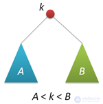 An AVL tree is, first and foremost, a binary search tree whose keys satisfy the standard property: the key of any node in the tree is not less than any key in that node's left subtree and not greater than any key in that node's right subtree. This means that a standard algorithm can be used to search for a given key in an AVL tree. To simplify the further discussion, we will assume that all keys in the tree are integers and do not repeat.
The distinguishing feature of an AVL tree is that it is balanced in the following sense: for any node of the tree, the height of its right subtree differs from the height of its left subtree by no more than one. It has been proven that this property is sufficient for the height of the tree to depend logarithmically on the number of its nodes: the height h of an AVL tree with n keys lies in the range from log2(n + 1) to 1.44 log2(n + 2) − 0.328. And since the basic operations on binary search trees (search, insertion, and deletion of nodes) depend linearly on its height, we get a guaranteed logarithmic dependence of the running time of these algorithms on the number of keys stored in the tree. Recall that randomized search trees guarantee balance only in a probabilistic sense: the probability of obtaining a strongly unbalanced tree for large n, although negligibly small, remains not equal to zero.
We will represent the nodes of an AVL tree with the following structure:
struct node // structure for representing the nodes of the tree
{
	int key;
	unsigned char height;
	node* left;
	node* right;
	node(int k) { key = k; left = right = 0; height = 1; }
};
The key field stores the node's key, the height field stores the height of the subtree rooted at this node, and the left and right fields are pointers to the left and right subtrees. The simple constructor creates a new node (of height 1) with the given key k.
Traditionally, the nodes of an AVL tree store not the height but the difference between the heights of the right and left subtrees (the so-called balance factor), which can take only three values: -1, 0, and 1. Note, however, that this difference is still stored in a variable whose size is at least one byte (unless you come up with some clever scheme for «efficiently» packing such values). Recall that the height h < 1.44 log2(n + 2), this means, for example, that for n=109 (one billion keys, more than 10 gigabytes of memory for storing the nodes) the height of the tree will not exceed h=44, which fits comfortably into that same single byte of memory as the balance factor. Thus, storing heights, on the one hand, does not increase the amount of memory allocated for the tree's nodes, and on the other hand, significantly simplifies the implementation of certain operations.
Let's define three helper functions related to height. The first is a wrapper for the height field, and it can also work with null pointers (with empty trees):
unsigned char height(node* p)
{
	return p?p->height:0;
}
The second computes the balance factor of a given node (and works only with non-null pointers):
int bfactor(node* p)
{
	return height(p->right)-height(p->left);
}
The third function restores the correct value of the height field for a given node (assuming that the values of this field in its right and left child nodes are correct):
void fixheight(node* p)
{
	unsigned char hl = height(p->left);
	unsigned char hr = height(p->right);
	p->height = (hl>hr?hl:hr)+1;
}
Note that all three functions are non-recursive, i.e., their running time is O(1).
The maximum height of an AVL tree for a given number of nodes:

where:
 (round up),
 (round down),
 (round down).
It is worth noting that the number of possible heights is, in practice, quite limited (with 32-bit addressing the maximum height is 45, with 48-bit addressing it is 68), so it may be better to precompute in advance all the values of the minimum number of nodes for each height using the recurrence formula for the Fibonacci tree:
 ,
,
 ,
,
 .
.
Intermediate values of the number of nodes will correspond to the previous (smaller) height.
In the process of inserting or deleting nodes in an AVL tree, a situation can arise where the balance factor of some nodes becomes equal to 2 or -2, i.e., an imbalance of the subtree occurs. To correct the situation, the rotations around particular tree nodes that we are already familiar with are applied. Recall that a simple right (left) rotation performs the following transformation of the tree:
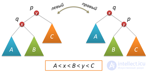
The code implementing the right rotation looks as follows (as usual, every function that modifies the tree returns the new root of the resulting tree):
node* rotateright(node* p) // right rotation around p
{
	node* q = p->left;
	p->left = q->right;
	q->right = p;
	fixheight(p);
	fixheight(q);
	return q;
}
The left rotation is a symmetric copy of the right one:
node* rotateleft(node* q) // left rotation around q
{
	node* p = q->right;
	q->right = p->left;
	p->left = q;
	fixheight(q);
	fixheight(p);
	return p;
}
Let's now consider an imbalance situation where the height of the right subtree of node p is 2 greater than the height of the left subtree (the reverse case is symmetric and is handled analogously). Let q be the right child of node p, and s be the left child of node q.
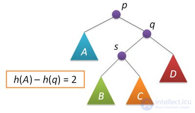
Analysis of the possible cases within this situation shows that, to correct the imbalance at node p, it is sufficient to perform either a simple left rotation around p, or the so-called big rotation to the left around the same p. A simple rotation is performed provided that the height of the left subtree of node q is greater than the height of its right subtree: h(s)≤h(D).
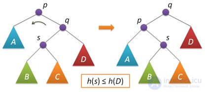
A big rotation is applied when h(s)>h(D), and in this case it reduces to two simple rotations — first a right rotation around q, and then a left rotation around p.
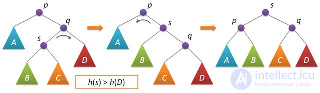
The code that performs balancing comes down to checking the conditions and performing the rotations:
node* balance(node* p) // balancing node p
{
	fixheight(p);
	if( bfactor(p)==2 )
	{
		if( bfactor(p->right) < 0 )
			p->right = rotateright(p->right);
		return rotateleft(p);
	}
	if( bfactor(p)==-2 )
	{
		if( bfactor(p->left) > 0  )
			p->left = rotateleft(p->left);
		return rotateright(p);
	}
	return p; // no balancing needed
}
The described rotation and balancing functions also contain neither loops nor recursion, which means they run in constant time, independent of the size of the AVL tree.
For an AVL tree, balancing a node is an operation that, when the difference in heights of the left and right subtrees = 2, changes the ancestor-descendant relationships in the subtree of this node so that the difference becomes <= 1, otherwise it changes nothing. This result is achieved by rotating the subtree of this node.
4 types of rotations are used:
1.Small left rotation 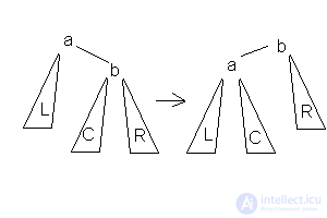 This rotation is used when the height of the b-subtree — height of L = 2 and the height of C <= the height of R.
2.Large left rotation 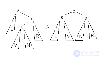 This rotation is used when the height of the b-subtree — height of L = 2 and the height of the c-subtree > the height of R.
3.Small right rotation 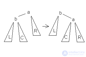 This rotation is used when the height of the b-subtree — height of R = 2 and the height of C <= the height of L.
4.Large right rotation 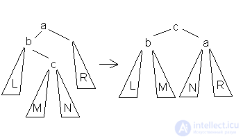 This rotation is used when the height of the b-subtree — height of R = 2 and the height of the c-subtree > the height of L.
In each case it is fairly easy to prove that the operation produces the required result and that the total height decreases by no more than 1 and cannot increase. It can also be noted that a large rotation is a combination of a right and a left small rotation. Because of the balance condition, the height of the tree is O(log(N)), where N is the number of nodes, so adding an element requires O(log(N)) operations.
Inserting a new key into an AVL tree is done, for the most part, the same way it is done in plain binary search trees: we descend down the tree, choosing the right or left direction of movement depending on the result of comparing the key at the current node and the key being inserted. The only difference is that when returning from the recursion (i.e., after the key has been inserted into either the right or the left subtree, and that subtree is balanced) balancing of the current node is performed. It can be strictly proven that the imbalance arising at any node along the path of movement from such an insertion does not exceed two, which means applying the balancing function described above is correct.
node* insert(node* p, int k) // insert key k into the tree with root p
{
	if( !p ) return new node(k);
	if( kkey )
		p->left = insert(p->left,k);
	else
		p->right = insert(p->right,k);
	return balance(p);
}
To verify that the implemented insertion algorithm matches the theoretical estimates for the height of AVL trees, a simple computational experiment was carried out. An array of randomly arranged numbers from 1 to 10000 was generated, then these numbers were sequentially inserted into an initially empty AVL tree, and the height of the tree was measured after each insertion. The results obtained were averaged over 1000 runs. The following graph shows the dependence on n of the average height (red line); the minimum height (green line); the maximum height (blue line). In addition, the upper and lower theoretical bounds are shown.
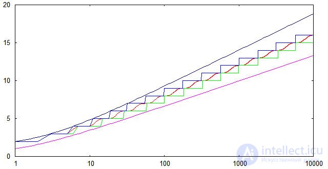
It can be seen that for random key sequences the experimentally found heights fall within the theoretical bounds, even with some margin. The lower bound is achievable (at least at some points) if the original sequence of keys is sorted in increasing order.
Going forward we will interpret the balance factor as the difference between the height of the left and right subtree, and the algorithm will be based on the TAVLTree type described above. When a node is inserted (as a leaf), it is assigned a zero balance. The process of inserting a node consists of three parts (this process is described by Niklaus Wirth in «Algorithms + Data Structures = Programs»):
We will return, as the result of the function, whether the height of the tree has decreased or not. Suppose the process returns to the parent from the left branch (recursion unwinds backward); then three cases are possible: { hl — height of the left subtree, hr — height of the right subtree }. Inserting a node into the left subtree will lead to
In the third situation it is necessary to determine the balance of the left subtree. If the left subtree of this node (Tree^.left^.left) is taller than the right one (Tree^.left^.right), a large right rotation is required, otherwise a small right rotation is enough. Similar (symmetric) reasoning can be applied for insertion into the right subtree.
Unfortunately, deleting nodes from an AVL tree is not as pleasant as with randomized search trees. It was not possible to find or come up with an approach based on merging (join) two trees. 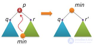 So the approach used almost everywhere as a basis was taken (and the one usually used when deleting nodes from a standard binary search tree). The idea is as follows: we find the node p with the given key k (if we don't find it, there is nothing to do), find the node min with the smallest key in the right subtree, and replace the node p being deleted with the found node min.
Several nuances arise during implementation. First of all, if the found node p has no right subtree, then by the AVL tree property, this node can have on the left either only a single child node (a tree of height 1), or node p is a leaf altogether. In both of these cases we simply need to delete node p and return, as the result, a pointer to the left child node of node p.
Now suppose p does have a right subtree. We find the minimum key in this subtree. By the binary search tree property, this key is located at the end of the left branch, starting from the root of the tree. We apply the recursive function:
node* findmin(node* p) // find the node with the minimum key in tree p
{
	return p->left?findmin(p->left):p;
}
Another helper function will handle deleting the minimum element from a given tree. Again, by the AVL tree property, the minimum element either has a single node hanging on the right, or nothing there at all. In both cases we simply need to return a pointer to the right node and, on the way back (when returning from the recursion), perform rebalancing. The minimum node itself is not deleted, since we will still need it.
node* removemin(node* p) // remove the node with the minimum key from tree p
{
	if( p->left==0 )
		return p->right;
	p->left = removemin(p->left);
	return balance(p);
}
Now everything is ready to implement deletion of a key from an AVL tree. First we find the required node, performing the same steps as when inserting a key:
node* remove(node* p, int k) // remove key k from tree p
{
	if( !p ) return 0;
	if( k < p->key )
		p->left = remove(p->left,k);
	else if( k > p->key )
		p->right = remove(p->right,k);
As soon as key k is found, we move on to plan B: we remember the roots q and r of the left and right subtrees of node p; we delete node p; if the right subtree is empty, we return a pointer to the left subtree; if the right subtree is not empty, we find the minimum element min in it, then extract it from there, attach q to min on the left, and what remains of r on the right, and return min after balancing it.
	else //  k == p->key
	{
		node* q = p->left;
		node* r = p->right;
		delete p;
		if( !r ) return q;
		node* min = findmin(r);
		min->right = removemin(r);
		min->left = q;
		return balance(min);
	}
When exiting the recursion, don't forget to perform balancing:
	return balance(p);
}
And that's basically all! Finding the minimum node and extracting it can, in principle, be implemented in a single function, but then one has to solve the (not very difficult) problem of returning a pair of pointers from the function. On the other hand, this saves one pass over the right subtree.
Obviously, the insertion and deletion operations (as well as the simpler search operation) run in time proportional to the height of the tree, since performing these operations involves descending from the root to the given node, and at each level a certain fixed number of actions is performed. And because the AVL tree is balanced, its height depends logarithmically on the number of nodes. Thus, the running time of all three basic operations is guaranteed to depend logarithmically on the number of nodes in the tree.
For simplicity, let us describe a recursive removal algorithm. If the node is a leaf, we remove it and call balancing on all its ancestors in order from parent to root. Otherwise we find the closest-valued node in the subtree of greater height (right or left) and move it to the place of the node being removed, calling the procedure to remove it in the process.
Let us prove that this algorithm preserves balance. To do this, we prove by induction on the height of the tree that after removing some node from the tree and the subsequent balancing, the height of the tree decreases by no more than 1. Base of the induction: Obviously true for a leaf. Induction step: Either the balance condition at the root (after removal the root may change) is not violated, in which case the height of this tree has not changed, or the strictly smaller of the subtrees has decreased => the height before balancing has not changed => afterwards it decreases by no more than 1.
Obviously, as a result of these actions the removal procedure is called no more than 3 times, since the node being removed on the second call is missing one of its subtrees. But finding the closest node each time requires O(N) operations. This makes an optimization possibility obvious: finding the closest node can be performed along the edge of the subtree, which reduces the complexity to O(log(N)).
The non-recursive algorithm is more complex than the recursive one.
To implement removal we will proceed from the same principle as with insertion: we find the node whose removal will not change its height. There are two cases:
To make it easier to understand, the algorithm given here does not contain any optimizations. Unlike the recursive algorithm, the found node to be removed is replaced with the value from the left subtree. This algorithm can be optimized in the same way as the recursive one (thanks to the fact that once the node to be removed is found, the direction of movement is known):
As already mentioned, if the node being removed is a leaf, it is removed, and the backward traversal of the tree proceeds from the parent of the removed leaf. If it is not a leaf, a «replacement» is found for it, and the backward traversal of the tree proceeds from the parent of the «replacement». Immediately after the element is removed, the «replacement» receives the balance of the removed node.
During backward traversal: if we arrive at the parent from the left, the balance increases by 1; if we arrive from the right, it decreases by 1.
This is done until, upon changing, the balance becomes equal to −1 or 1 (note the difference from element insertion!): in this case such a change in balance indicates that the delta-height of the subtrees is unchanged. Rotations occur according to the same rules as with insertion.
Let us denote:
If the rotation is performed during insertion of an element, then the balance of Pivot equals either 1 or −1. In this case, after the rotation the balances of both are set equal to 0. On removal everything is different: the balance of Pivot may become equal to 0 (this is easy to verify).
Here is a summary table of the dependence of the final balances on the direction of rotation and the initial balance of the Pivot node:
| Rotation direction | Old Pivot.Balance | New Current.Balance | New Pivot.Balance |
|---|---|---|---|
| Left or Right | -1 or +1 | 0 | 0 |
| Right | 0 | -1 | +1 |
| Left | 0 | +1 | -1 |
Pivot and Current are the same as before, but a third participant in the rotation is added. Let us denote it «Bottom»: this is (in a double right rotation) the left child of Pivot, and in a double left rotation — the right child of Pivot.
With this rotation — Bottom always ends up with a balance of 0, but the resulting balances for Pivot and Current depend on Bottom's initial balance.
Here is a summary table of the dependence of the final balances on the direction of rotation and the initial balance of the Bottom node:
| Direction | Old Bottom.Balance | New Current.Balance | New Pivot.Balance |
|---|---|---|---|
| Left or Right | 0 | 0 | 0 |
| Right | +1 | 0 | -1 |
| Right | -1 | +1 | 0 |
| Left | +1 | -1 | 0 |
| Left | -1 | 0 | +1 |
From the formula given above, the height of an AVL tree will never exceed the height of a perfectly balanced tree by more than 45%. For large  the estimate
  holds. Thus, performing the basic operations requires on the order of
  comparisons. It has been found experimentally that one rebalancing occurs for every 2 insertions and every 5 deletions.
A splay tree (splay tree) or skewed tree is a binary search tree in which the balance property is maintained. This tree belongs to the class of «self-adjusting trees», which maintain the necessary branching balance of the tree in order to ensure that search, insertion, and deletion operations run in time logarithmic in the number of stored elements. This is achieved without using any additional fields in the tree nodes (as, for example, in red-black trees or AVL trees, where nodes store, respectively, the color of the node and the depth of the subtree). Instead, «splay operations» (splay operation), which include rotations, are performed on every access to the tree. The amortized cost (amortized) per operation on the tree is  .
.
The splay tree was invented by Robert Tarjan and Daniel Sleator in 1983.
Splay tree (Splay-tree) — is a binary search tree. It allows data that has been used recently to be found faster. It belongs to the category of mergeable trees. The splay tree was invented by Robert Tarjan and Daniel Sleator in 1983.
In order for access to recently found data to be faster, this data needs to be located closer to the root. We can achieve this using various heuristics:
 , where
  — is the found node,
  — is its ancestor, until becomes the root of the tree. However, one can construct such a sequence of operations that the amortized access time to a node will be
  .
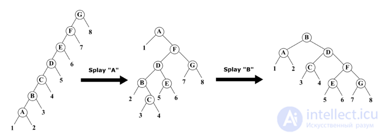
.Example: When using the "move to root" operation sequentially for nodes  and
and  6 rotations are required each time, whereas using the "splay" operation for node 3 rotations are enough.
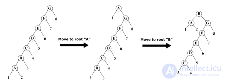
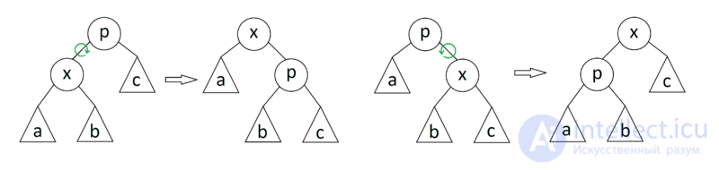
"splay" is split into 3 cases:
zig
If — is the root of the tree with child , then we perform a single rotation around the edge , making the root of the tree. This case is an edge case and is performed only once at the end, if the initial depth of was odd.
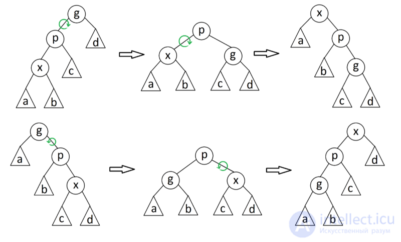
zig-zig
If — is not the root of the tree, and and — are either both left or both right children, then we perform a rotation of the edge  , where
  is the parent of , and then a rotation of the edge .
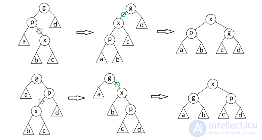
zig-zag
If — is not the root of the tree and — is the left child, and — is the right one, or vice versa, then we perform a rotation around the edge , and then a rotation of the new edge  , where — is the former parent of .
This operation takes  time, where
  — is the length of the path from to the root.
This operation is performed as for an ordinary binary tree, except that afterwards the splay operation is run.
We have two trees  and
and  , where it is assumed that all elements of the first tree are less than the elements of the second. We run splay from the largest element in tree (let this be element
  ). After this, the root contains element , and it has no right child. We make the right subtree of and return the resulting tree.
We run splay from element and return two trees obtained by cutting off the right or left subtree from the root, depending on whether the root contains an element greater than, or not greater than, .
We run split(tree, x), which returns to us trees and , which we attach to as the left and right subtrees respectively.
We run splay from element and return Merge of its children.
Amortized analysis of a splay tree is carried out using the potential method. We call the potential of the tree in question the sum of the ranks of its nodes. The rank of node — is a quantity denoted  and equal to
  , where
  — is the number of nodes in the subtree rooted at .
| Lemma: |
The amortized time of the splay operation on node in the tree rooted at  does not exceed does not exceed  |
| Proof: |
 |
|
Let us analyze each step of the splay operation. Let Let us go through the cases depending on the type of step: zig. Since one rotation is performed, the amortized running time of the step is zig-zig. Two rotations are performed, the amortized running time of the step is Further, since We claim that this sum does not exceed From the figure it is clear that zig-zag. Two rotations are performed, the amortized running time of the step is We claim that this sum does not exceed In total, we obtain that the amortized time of a zig-zag step does not exceed , since the tripled ranks of the intermediate nodes cancel out (they enter the sum both with a plus and a minus sign). Then the total running time of splay is  , where , where  — is the number of elements in the tree. — is the number of elements in the tree. |
 |
| Theorem: |
|
If |
| Proof: |
|
|
It is known that Let Let us denote by Let  — is the root of the — is the root of the  -tree, it is obvious that -tree, it is obvious that 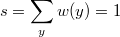 , therefore , therefore  . Hence . Hence  , q.e.d. , q.e.d. |
|
| Theorem (on nearby queries in a splay tree): |
|
Suppose keys |
| Proof: |
|
|
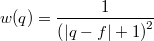
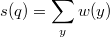
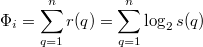
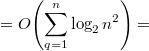
To prove the theorem we use the potential method:
By the condition,
Let us introduce the following notation:
Let The latter is true because for a fixed From the definition of the size of a node it follows that Also note that for any Then, using the estimates obtained, let us find the change in the potential of the splay tree after
The first inequality is true because the maximum value of the potential is achieved at Let us denote by
Let us prove that this definition of potential satisfies the condition of the theorem on the potential method. For any Then, substituting the found values into the formula   . . |
|
This theorem shows that splay trees support fairly efficient access to keys that are located close to some fixed key.
A splay tree by implicit key is completely analogous to a treap by implicit key; the implicit key will likewise be the number of tree elements smaller than the given one. Similarly, we will store an auxiliary quantity — the number of nodes in the subtree. To the operations already presented for the treap, splay is added, but recomputing in it is trivial, since we know exactly where the modified subtrees are moved.
Treap or cartesian tree (Treap) — is a data structure combining a binary search tree and a binary heap (hence its second name: treap (tree + heap), also known as dermaid (tree + pyramid), and there is also the name "kuchevo" (heap + tree)).
Treap — is a binary tree, in whose nodes are stored:
A reference to the parent node is not mandatory; it is only desirable for a linear tree-construction algorithm.
A treap is not self-balancing in the usual sense, and it is used for the following reasons:
Disadvantages of the treap:
More formally, this is a binary tree whose nodes store pairs  , where
  — is the key, and
  — is the priority. It is also a binary search tree by and a heap by . Assuming that all and all are distinct, we obtain that if some element of the tree contains
  , then for all elements in the left subtree
  , for all elements in the right subtree
  , and also both in the left and in the right subtree we have:
  .
.
Treaps were proposed by Siedel (Siedel) and Aragon (Aragon) in 1996.
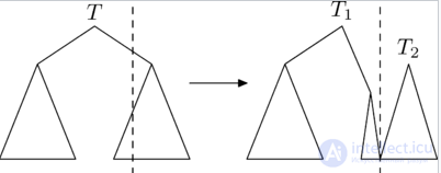
The split operation
The  (split) operation allows us to do the following: split the original tree
  by key
  . It will return a pair of trees
  such that tree
  contains keys less than , and tree
  contains all the rest:
 .
.
This operation works as follows.
Let us consider the case in which we need to split the tree by a key greater than the root's key. Let us look at how the resulting trees and will be structured:
: the left subtree of will coincide with the left subtree of . To find the right subtree of , we need to split the right subtree of into  and
and  by key and take . will coincide with .
The case in which we need to split the tree by a key less than or equal to the key at the root is considered symmetrically.
Treap, Treap split(t: Treap, k: int):
  if t ==
return  ,
,
else if k > t.x
t1, t2 = split(t.right, k)
    t.right = t1
    return t, t2
else
t1, t2 = split(t.left, k)
    t.left = t2
    return t1, t
Let us estimate the running time of the operation. During execution, one operation is called for a tree of height at least one less, and  more operations are performed. Then the total complexity of this operation is equal to
  , where
  — is the height of the tree.
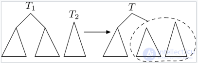
The merge operation
Let us consider the second operation on treaps —  (merge).
Using this operation, two treaps can be merged into one. Moreover, all keys in the first (left) tree must be smaller than the keys in the second (right) tree. The result is a tree that contains all the keys from the first and second trees: 
Let us consider how this operation works. Suppose we need to merge trees and . Then, obviously, the resulting tree has a root. The root will be the node from or with the highest priority . But the node with the highest among all nodes of trees and can only be either the root of , or the root of . Let us consider the case where the root of has a greater than the root of . The case where the root of has a greater than the root of is symmetric to this one.
If the of the root of is greater than the of the root of , then it will be the root. Then the left subtree of will coincide with the left subtree of . On the right, we need to attach the merge of the right subtree of and tree .
Treap merge(t1: Treap, t2: Treap):
  if t2 ==
    return t1
  if t1 ==
    return t2
  else if t1.y > t2.y
    t1.right = merge(t1.right, t2)
    return t1
  else
    t2.left = merge(t1, t2.left)
    return t2
Reasoning similarly to the operation, we conclude that the complexity of the operation equals , where — is the height of the tree.
The  operation adds to tree an element , where
  — is the key, and
  — the priority.
Let us imagine that element is a treap consisting of a single element, and in order to add it to our treap , obviously we need to merge them. But may contain keys both smaller and larger than key , so first we need to split by key .
 .
. .
. .), but stop at the first element whose priority value turns out to be less than . on the found element (on the element together with its entire subtree) and are recorded as the left and right children of the element being added.
In the first implementation is used twice, while in the second implementation merging is not used at all.
The  operation removes from tree the element with key .
 . from the first tree, that is, the leftmost child of tree .
 .), and look for the element to be removed. on its left and right children procedure in place of the element being removed.
In the first implementation is used once, while in the second implementation splitting is not used at all.
Suppose we know the pairs  from which the treap needs to be built, and it is also known that
  .
.

Let us sort all priorities in decreasing order in and pick the first of them, let it be  . Let us make
  the root of the tree. Doing the same with the remaining nodes, we get the left and right children of . On average, the height of a treap is
  (see below), and at each level we performed
  operations. This means such an algorithm runs in .
Let us sort the pairs in decreasing order of  and put them in a queue. First, we take the first
  elements out of the queue and merge them into a tree, and put it at the end of the queue, then we do the same with the next two, and so on. In this way, we will first merge
  trees of size
  , then
  trees of size , and so on. In doing so, halving the size of the queue will cost us a total of time on merges, and there will be a total of such halvings. This means the total running time of the algorithm will be .
We will build the tree from left to right, that is, starting from  to
to  , while keeping track of the last added element . It will be the rightmost one, since it will have the maximum key, and by keys a treap is a binary search tree. When adding
  , we try to make it the right child of ; this should be done if
  , otherwise we step up to the ancestor of the last element and look at its value . We climb up until the priority in the element being examined is less than the priority of the element being added, after which we make its right child, and make the previous right child the left child of .
Note that we visit each node at most twice: when it is directly added and, while climbing up (since after this the node will lie in someone's left subtree, and we only climb up along the right side). It follows that the construction runs in .
We have already found that the complexity of operations on a treap depends linearly on its height. In fact, the height of a treap can be linear relative to its size. For example, the height of a treap built on the set of keys  will be equal to . To avoid such cases, it turns out to be useful to choose the priorities of the keys randomly.
| Theorem: | ||||||
|
In a treap of |
||||||
| Proof: | ||||||
 |
||||||
|
We will assume that all chosen priorities First, let us introduce some notation:
With this notation, the depth of a node can be written as the number of ancestors:
Now we can express the expected value of the depth of a specific node:
To compute the average depth of nodes, we need to compute the probability that node Let us introduce a new notation:
Since the priority distribution is uniform, each vertex among
Substituting the latter into our formula for the expectation, we get:
 . . |
||||||
 |
Thus, the average running time of the operations and will be  .
.
[[b66]]
[[b8344]]
 and
and  (since only nodes
  . The rank of node
  . Therefore,
  .
. . Since after the rotations the subtree rooted at
  . Using this equality, we obtain:
  , since
  .
. , we obtain that
  .
. , that is, that
  . Let us transform the resulting expression as follows:
  .
. , hence the sum of the expressions under the logarithms does not exceed one. Next, consider the sum of logarithms
  . For
. For  the product
  by the inequality between means does not exceed
  . And since the logarithm is an increasing function,
  , which is the required inequality.
 . Since
  . Further, since
  .
. , that is, that
  . But, since
  - similarly to what was proved earlier, which is what was to be proved.
 .
. queries are performed on keys
  stored in a splay tree, and
  -th key, where
  , then the total running time does not exceed
  , where
  ,
,  — is the Shannon entropy
 — is the Shannon entropy.
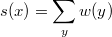 — be the number of nodes in the subtree rooted at
  — the rank of the node.

 , then
  .
.

 are stored in a splay tree. Let us fix one of the keys
  . Suppose
  , where
  — is the value at the node accessed by the
  .
.
 .
. the quantity
  .
. , where
  — are the nodes of the subtree rooted at
  — the rank of the node.
 .
. — be the weight of the tree. Then
  .
. , the series converges.
 .
. to
to  it holds that
  , since the maximum value of the denominator in the definition of
  is achieved when
  and
and  or vice versa.
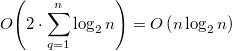 .
. , and the minimum at
  , which means the change in potential does not exceed the difference of these quantities.
 .
. , since
  , and
, and  , as was shown above. Since the number of operations per query is
  , then
  and
and  , where
  — is the function from the theorem on the potential method, equal in this case to
  . Therefore, the potential satisfies the condition of the theorem.
 .
. — the node with the
 — the depth of node
  ;
;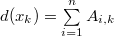 .
. — here we used the linearity of expectation, and the fact that
  for the indicator variable
  (
( — is the probability of the event
  ).
). .
. — the set of keys
  or
or  , depending on
  or
or  .
.  denote the same thing, and their cardinality equals
  .
. ,
,  — is the root. Then, if
  or
or  , hence,
  . In this case
  .
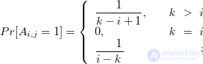
.

 (here we used the inequality
 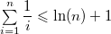 )
) differs from
  by a constant factor, therefore
  .
.
Comments