
Lecture
A search tree with minimal height is precisely what is called balanced, i.e., one in which the heights of the left and right subtrees differ by no more than one. It is called balanced, presumably, because such a tree requires, on average, the smallest number of operations for a search.
The running time of the basic operations on a search tree is linearly dependent on its height. But different search trees can be built from the same set of keys, as shown in Fig. 3.
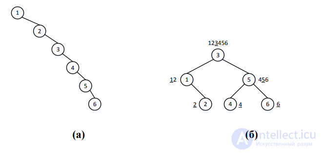
Fig. 3. Different search trees built from the same set of keys
In the example shown in Fig. 3, both trees are built from the same
set of keys, but the height of the first tree is greater, so the running time of operations on it will be greater. For example, when searching for the node with key 6, case (a) requires examining all six nodes, whereas case (b) requires examining only three nodes: 3->5->6. The second tree is better balanced than the first. In this case
the advantage of a binary search tree over an ordinary binary tree is clearly visible. If the tree in Fig. 3(b) were not a search tree, then searching for the node with key 6 would require examining anywhere from 4 to 6 nodes, depending on the traversal order of the tree. But in a search tree, movement during a search only goes downward,
so the number of steps is bounded by the height of the tree. The more nodes there are in the tree, the more evident the advantage of a search tree over an ordinary binary tree becomes, provided the search tree is well balanced. How do you build a search tree of minimal height? If the set of keys is known in advance, it must be sorted. The root of a subtree becomes the node whose key value is the median of that set. For a sorted set containing an odd number of keys, this is the key located exactly in the middle of the set. For the set 1,2,3,4,5,6 from the example in Fig. 3, which contains an even number of keys, either the key with value 3 or the key with value 4 can be chosen as the median. For definiteness, let's choose 3. The node with this key will be the root of the tree.
Next, keys smaller than 3 go into the left subtree, and keys greater than 3 go into the right subtree. To build the left and right subtrees, we repeat the same procedure on the corresponding sets of keys. This continues until all keys have been included in the tree. In Fig. 3(b), for each node, the set of keys for which the tree rooted at that node is built is shown, with the median of that set highlighted, since it is the one that ends up at the root.
The tree shown in Fig. 3(b) is perfectly balanced, meaning that for each of its nodes, the number of nodes in the left and right subtrees differs by no more than 1. Such a tree can be built for any set of keys. It suffices to note that, since the median is chosen at each step of building the tree, the set of keys is split into two parts, and the number of keys in them can differ by no more than 1.
The complete set of keys is not always known in advance. If keys arrive one at a time, the construction of the search tree will depend on the order in which they arrive. If, for example, the keys arrive in the order 1,2,3,4,5,6, the result is the tree shown in Fig. 3(a). The height of such a tree is maximal for this set of keys, and consequently the running time of operations on it will also be maximal. Therefore, when a new node is added, the tree may need to be rebuilt in order to reduce its height while keeping the same set of nodes. Maintaining perfect balance is difficult. If, when a new node is added, the number of nodes in the left and right subtrees of some node in the tree comes to differ by more than 1, then the tree will no longer be
perfectly balanced, and it will need to be rebuilt in order to restore the properties of a perfectly balanced
search tree. Therefore, the balance requirements for a tree are usually less strict.
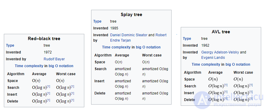
Let's consider three main types of balanced search trees:
For AVL trees, balance is determined by the difference between the heights of the right and left subtrees of any node. If the absolute value of this difference does
not exceed 1, the tree is considered balanced. This condition is checked after every node insertion or deletion, and a minimal set of tree-restructuring operations is defined that restores the balance property whenever it has been violated. In red-black trees, each node has an additional property – its color, red or black. Constraints are imposed on the tree regarding the placement and number of nodes depending on color, and a set of tree-restructuring operations is defined for the case where these constraints are violated after a node is inserted or deleted. Whereas AVL trees impose fairly strict balance conditions, and the tree often has to be restructured as nodes are added, in a red-black tree the heights of the left and right subtrees of any node can differ by at most a factor of two. Finally, the third type of balanced search tree under consideration is self-adjusting trees. Unlike the two previous types, these trees have no restrictions on node placement at all, and balance is achieved on average by moving each node to the root of the tree every time an operation is performed on it. However, there is a chance that the tree may turn out to be unbalanced, as, for example, in Fig. 3(a).
An AVL tree is a search tree in which, for every node, the heights of the left and right subtrees differ by no more than 1. This data structure was developed by the Soviet scientists Georgy Maximovich Adelson-Velsky and Evgenii Mikhailovich Landis in 1962. The abbreviation AVL corresponds to the first letters of these scientists' surnames. AVL trees were originally invented to organize search in chess programs. The Soviet chess program «Kaissa» became the first official world champion in 1974.
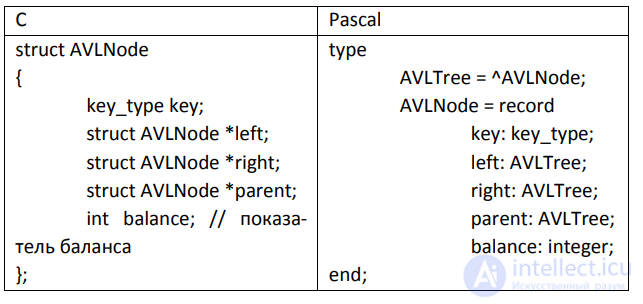
In each node of an AVL tree, in addition to the key, the data, and pointers to the left and right subtrees (the left and right children), a balance factor is stored – the difference between the heights of the right and left subtrees. In some implementations, this factor may instead be computed separately while processing the tree, whenever it is needed. Fig. 4(a) shows an example of an AVL tree. Thus, it turns out that in an AVL tree the balance factor balance for every node, including the root, does not exceed 1 in absolute value. Fig. 4(b) shows an example of a tree that is not an AVL tree, since at one of its nodes the balance is violated, i.e., |balance|>1. From here on, for AVL trees we will indicate the value of the balance factor at the node.
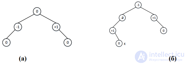
Fig. 4. (a) an example of an AVL tree; (b) an example of a tree that is not an AVL tree: at node X the balance is violated
Two extreme cases of AVL trees are: (a) a perfect tree – all nodes have a balance factor of 0; (b) a Fibonacci tree – all nodes except the leaves have a balance factor of +1, or all nodes except the leaves have a balance factor of –1. Examples are shown in Fig. 14
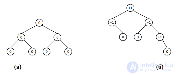
Fig. 14. Extreme cases of AVL trees: (a) a perfect tree; (b) a Fibonacci tree
It is not possible to build a perfect tree for every set of keys, just as it is not possible to build a Fibonacci tree for every set of keys. But these trees make it possible to estimate the range of possible heights of AVL trees. A perfect tree is a special case of a perfectly balanced tree, so it has the minimum possible height for a given number of nodes. A Fibonacci tree, in contrast, has the maximum possible height for a given number of nodes, provided the properties of an AVL tree are preserved.
Basic operations for AVL trees
AVL trees were historically the first example of the use of balanced search trees. Today, red-black trees (RB-trees) are more popular. Rudolf Bayer, a German scientist, is considered the inventor of the red-black tree. This data structure got its name from a 1978 paper by Leonidas Guibas and Robert Sedgewick. RB-trees are binary search trees in which each node stores an additional field, color, indicating its color – red or black – and which satisfy the properties listed below.
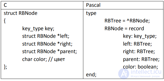
We will assume that if left or right equal NULL, these are «pointers» to dummy leaves. Thus, all nodes are internal (non-leaf) nodes.
Properties of RB-trees:
1. every node is either red or black;
2. every (dummy) leaf is black;
3. if a node is red, then both of its children are black;
4. all paths from the root to any dummy leaf contain the same number of black nodes;
5. the root is black.
Definition 4: The black height of a node is the number of black nodes on the path from that node to a node whose children are both dummy leaves.
The node itself is not included in this count. For example, for the tree shown in Fig. 15, the black height of the root equals 2.
Definition 5: The black height of a tree is the black height of its root.
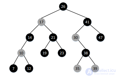
Fig. 15. An example of a red-black tree
Basic operations for RB-trees
A self-adjusting tree is a binary search tree that, unlike the two previous types of trees, does not contain additional service fields in its data structure (balance, color, etc.). It allows data that has been used recently to be found faster. The self-adjusting tree
was invented by Robert Tarjan and Daniel Sleator in 1983.
The idea behind self-adjusting trees is based on the principle of moving the found node to the root of the tree. This operation is called splay(T, k), where k is the key and T is the binary search tree.
After the operation splay(T, k) is performed, the binary tree T is restructured, while remaining a search tree, such that:
Thus, searching for a node in a self-adjusting tree essentially amounts to performing the splay operation. The move-to-front heuristic (moving the found node to the root) is based on the assumption that if the same element is needed again soon, it will be found faster.
Definition 6: The dictionary operations on a tree are the basic operations: search, insertion, and deletion.
Basic operations
In general, comparing the three types of trees discussed is difficult, since the best type of tree may differ for different tasks and different data sets. Trees can be compared using different criteria: implementation complexity, theory, and practice.
In terms of implementation complexity, the simplest is the AVL tree, and the most complex are RB-trees, since many non-trivial cases have to be considered when inserting and deleting a node. In theory, the upper bounds for all three types of trees are roughly the same. Restoring the properties of both an AVL tree and an RB-tree after an insertion requires no more than two rotations. But after deleting a node from an RB-tree, no more than three rotations are required, whereas in an AVL tree, after deleting a node, the number of rotations required can be as large as the height of the tree (from leaf to root). Therefore, the deletion operation is more efficient in RB-trees, which is why they are
more widely used.
Self-adjusting trees differ substantially from AVL and RB-trees, since no restrictions whatsoever are imposed on the structure of the tree. The search operation on the tree modifies the tree itself, so when different nodes are accessed, a self-adjusting tree may work more slowly. Moreover, in the course of operation the tree may end up completely unbalanced. But it has been proven that if the probabilities of accessing the nodes are fixed, a self-adjusting tree will work asymptotically no slower than the other two types of trees discussed. The absence of extra fields gives it an advantage in memory usage.
Various kinds of balanced search trees are used, in particular, in system software, for example, in operating system kernels. The referenced article presents the results of tests simulating a certain real-world load on search trees. Given that virtual address tables in Linux are often implemented using binary search trees, the authors instrumented several applications to obtain the sequence of their accesses to the virtual memory subsystem, and then used these sequences to emulate the load on binary trees in the operating system kernel. For example, it is shown that if, when the Mozilla browser uses virtual memory, the virtual memory manager were to use self-adjusting trees, the advantage of this type of tree in running time over AVL and RB-trees would be a minimum of 2 times and a maximum of 3.4 times.
The article also shows which type of tree is best to use in which situation. If the input data is completely randomized, the best option turns out to be general-purpose search trees – unbalanced ones. If the input data is mostly randomized but ordered sets periodically occur, then RB-trees should be chosen. If ordered data predominates during insertion, then AVL trees turn out to be better when subsequent access to the elements is randomized, while self-adjusting trees are better when subsequent access is sequential or clustered.

Comments