
Lecture
The RMQ problem occurs very often in competitive and applied programming.
The abbreviation RMQ stands for Range Minimum (Maximum) Query – a query for the minimum (maximum) on a segment of an array. For definiteness we will consider the operation of taking the minimum.
Let an array A[1..n] be given. We need to be able to answer queries of the form «find the minimum on the segment from the i-th element to the j-th».
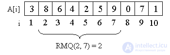
Let us consider as an example the array A = {3, 8, 6, 4, 2, 5, 9, 0, 7, 1}.
For example, the minimum on the segment from the second element to the seventh is equal to two, that is, RMQ(2, 7) = 2.
An obvious solution comes to mind: we will find the answer to each query simply by running through all the elements of the array lying on the segment we need. Such a solution, however, is not the most efficient. Indeed, in the worst case we will have to run through O(n) elements, i.e. the time complexity of this algorithm is O(n) per query. However, the problem can be solved more efficiently.
First, let's clarify the statement of the problem.
What does the word static mean in the title of the article? The RMQ problem is sometimes posed with the possibility of changing elements of the array. That is, to the query of taking the minimum is added the possibility of changing an element, or even changing elements on a segment (for example, increasing all elements on a subsegment by 3). This variant of the problem, called dynamic RMQ, I will consider in subsequent articles.
I will note here that the RMQ problem is subdivided into offline and online versions. In the offline variant there is the possibility of first obtaining all the queries, analyzing them in some way, and only then giving an answer to them. In the online formulation, queries are given one after another, i.e. the next query arrives only after the answer to the previous one. Note that having solved RMQ in the online formulation, we immediately obtain a solution for offline RMQ as well, although there may exist a more efficient solution for offline RMQ that is not applicable to the online formulation.
In this article we will consider static online RMQ.
To evaluate the efficiency of an algorithm, let us introduce one more time characteristic – the preprocessing time. In it we will account for the time spent on preparation, i.e. precomputing some information necessary to answer the queries.
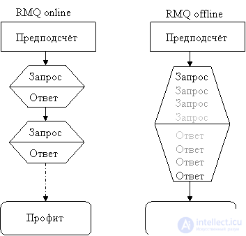
It might seem: why do we need to single out preprocessing separately? Here's why. Let us give one more solution to the problem.
Before we start answering queries, let's simply compute the answer for every segment! That is, let's build an array P[n][n] (from now on I will use C-like syntax, though I will number the array A from one for simplicity of implementation), where P[i][j] will equal the minimum on the segment from i to j. Moreover, let's compute this array even in O(n3) – in the dumbest way, running through all the elements for each segment. Why are we doing this? Suppose the number of queries q is much greater than n3. Then the total running time of our algorithm is O(n3) + q * O(1) = O(q), i.e. the preprocessing time will, by and large, not affect the overall running time of the algorithm. But thanks to the precomputed information, we have learned to answer a query in time O(1) instead of O(n). It is clear that O(q) is better than O(qn).
On the other hand, when q < n3 the preprocessing time will play its role, and in the algorithm given it – O(n3) – is unfortunately too large, even though it can be reduced (think how) to O(n2).
From this point on we will denote the time characteristics of an algorithm as (P(n), Q(n)), where P(n) – is the time for precomputation and Q(n) – is the time to answer one query.
So, we have two algorithms. One works in (O(1), O(n)), the second – in (O(n2), O(1)). Let's learn to solve the problem in (O(nlogn), O(1)), where logn – is the binary logarithm of n.
A lyrical digression. Note that any number can be taken as the base of the logarithm, since logan always differs from logbn by exactly a constant factor. The constant, as we remember from the school algebra course, equals logab.
So, we have arrived at the next step:
A Sparse Table – is a table ST[][] such that ST[k][i] is the minimum on the half-interval [A[i], A[i+2k]). In other words, it contains the minimums on all segments whose length is a power of two.
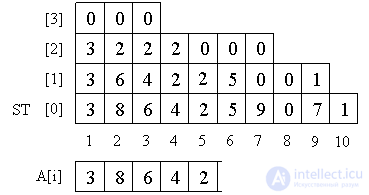
Let's compute the array ST[k][i] as follows. It is clear that ST is simply our array A. Next let's use an obvious property:
ST[k][i] = min(ST[k-1][i], ST[k-1][i + 2k — 1]). Thanks to it we can first compute ST , then ST and so on.
Note that our table has O(nlogn) elements, because the level numbers must not exceed logn, since for large values of k the length of the half-interval becomes greater than the length of the whole array and it makes no sense to store the corresponding values. And at each level there are O(n) elements.
Another lyrical digression: It is easy to notice that we are left with many unused elements of the array. Wouldn't it be better to store the table differently so as not to waste memory in vain? Let us estimate the amount of unused memory in our implementation. On the i-th row the number of unused elements is 2i – 1. Hence, in total the number of unused elements is Σ(2i – 1) = O(2logn) = O(n), i.e. in any case we will need on the order of O(nlogn) – O(n) = O(nlogn) space to store the Sparse Table. So we need not worry about unused elements.
And now the main question: why did we compute all this? Note that any segment of the array can be split into two overlapping subsegments whose length is a power of two.
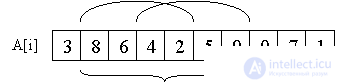
We get a simple formula for computing RMQ(i, j). If k = log(j – i + 1), then RMQ(i, j) = min(ST(i, k), ST(j – 2k + 1, k)). Thus, we obtain an algorithm running in (O(nlogn), O(1)). Hooray!
…almost obtain it. How were we going to compute the logarithm in O(1)? The simplest way is to precompute it as well for all values not exceeding n. It is clear that the asymptotics of the preprocessing will not change because of this.
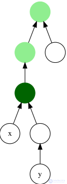
Finding it in O (sqrt (N)) and O (log N) with preprocessing O (N). Let a tree G be given. Queries of the form (V1, V2) arrive as input; for each query it is required to find their lowest common ancestor, i.e. the vertex V that lies on the path from the root to V1, on the path from the root to V2, and among all such vertices the lowest one must be chosen. In other words, the sought vertex V is an ancestor of both V1 and V2, and among all such common ancestors the lowest one is chosen. Obviously, the lowest common ancestor of vertices V1 and V2 is their common ancestor lying on the shortest path from V1 to V2. In particular, for example, if V1 is an ancestor of V2, then V1 is their lowest common ancestor.
In English this problem is called the LCA problem - Least Common Ancestor.
Before answering queries, let's perform so-called preprocessing. Let's run a depth-first search from the root, which will build a list of visited vertices Order (the current vertex is added to the list upon entering that vertex, and also after each return from a child of it); it is easy to see that the resulting size of this list will be O (N). And let's build an array First[1..N], in which for each vertex the position in the array Order at which this vertex stands is indicated, i.e. Order[First[I]] = I for all I. Also, using depth-first search, let's find the height of each vertex (the distance from the root to it) - H[1..N].
How do we now answer queries? Let there be a current query - a pair of vertices V1 and V2. Let's consider the list Order between the indices First[V1] and First[V2]. It is easy to see that the sought LCA (V1, V2) will also be located in this range, as well as a number of other vertices. However, LCA (V1, V2) will differ from the other vertices in that it will be the vertex with the smallest height.
Thus, in order to answer a query, we simply need to find the vertex with the smallest height in the array Order in the range between First[V1] and First[V2]. Thus, the LCA problem reduces to the RMQ problem ("minimum on a segment"). And the latter problem is solved with the help of data structures (see the RMQ problem).
If we use sqrt decomposition, we can obtain a solution that answers a query in O (sqrt (N)) and performs preprocessing in O (N).
If we use a segment tree, we can obtain a solution that answers a query in O (log (N)) and performs preprocessing in O (N).
Here is a ready-made implementation of LCA using a segment tree:
typedef vector < vector<int> > graph;
typedef vector<int>::const_iterator const_graph_iter;


vector<int> lca_h, lca_dfs_list, lca_first, lca_tree;
vector<char> lca_dfs_used;

void lca_dfs (const graph & g, int v, int h = 1)
{
	lca_dfs_used[v] = true;
	lca_h[v] = h;
	lca_dfs_list.push_back (v);
	for (const_graph_iter i = g[v].begin(); i != g[v].end(); ++i)
		if (!lca_dfs_used[*i])
		{
			lca_dfs (g, *i, h+1);
			lca_dfs_list.push_back (v);
		}
}

void lca_build_tree (int i, int l, int r)
{
	if (l == r)
		lca_tree[i] = lca_dfs_list[l];
	else
	{
		int m = (l + r) >> 1;
		lca_build_tree (i+i, l, m);
		lca_build_tree (i+i+1, m+1, r);
		if (lca_h[lca_tree[i+i]] < lca_h[lca_tree[i+i+1]])
			lca_tree[i] = lca_tree[i+i];
		else
			lca_tree[i] = lca_tree[i+i+1];
	}
}

void lca_prepare (const graph & g, int root)
{
	int n = (int) g.size();
	lca_h.resize (n);
	lca_dfs_list.reserve (n*2);
	lca_dfs_used.assign (n, 0);

	lca_dfs (g, root);

	int m = (int) lca_dfs_list.size();
	lca_tree.assign (lca_dfs_list.size() * 4 + 1, -1);
	lca_build_tree (1, 0, m-1);

	lca_first.assign (n, -1);
	for (int i = 0; i < m; ++i)
	{
		int v = lca_dfs_list[i];
		if (lca_first[v] == -1)
			lca_first[v] = i;
	}
}

int lca_tree_min (int i, int sl, int sr, int l, int r)
{
	if (sl == l && sr == r)
		return lca_tree[i];
	int sm = (sl + sr) >> 1;
	if (r <= sm)
		return lca_tree_min (i+i, sl, sm, l, r);
	if (l > sm)
		return lca_tree_min (i+i+1, sm+1, sr, l, r);
	int ans1 = lca_tree_min (i+i, sl, sm, l, sm);
	int ans2 = lca_tree_min (i+i+1, sm+1, sr, sm+1, r);
	return lca_h[ans1] < lca_h[ans2] ? ans1 : ans2;
}

int lca (int a, int b)
{
	int left = lca_first[a],
		right = lca_first[b];
	if (left > right)  swap (left, right);
	return lca_tree_min (1, 0, (int)lca_dfs_list.size()-1, left, right);
}

int main()
{
	graph g;
	int root;
	... read the graph ...

	lca_prepare (g, root);

	for (;;)
	{
		int v1, v2; // a query has arrived
		int v = lca (v1, v2); // answer to the query
	}
}
The simplest, naive algorithm for finding the lowest common ancestor — compute the depth of vertices u and v and gradually climb up the tree from each vertex until a common vertex is found:
Procedure LCA(u, v):
    h1 := depth(u)          // depth(x) = the depth of vertex x
    h2 := depth(v)

    while h1 ≠ h2:
       if h1 > h2:
          u := parent(u)
          h1 := h1 - 1
       else:
          v := parent(v)
          h2 := h2 - 1

    while u ≠ v:
       u := parent(u)       // parent(x) = the direct ancestor of vertex x
       v := parent(v)

    return u
The running time of this algorithm is O(h), where h — is the height of the tree. In addition, preprocessing requiring O(n) time may be needed to find the direct ancestor for all vertices of the tree (but usually this structure already exists on the tree).
However, there are faster algorithms:
The problem of computing the lowest common ancestors of classes in an inheritance hierarchy arises in the implementation of object-oriented programming systems ( Aït-Kaci et al. 1989 ). The LCA problem also finds application in models of complex systems used in distributed computing ( Bender et al. 2005 ).
| Problem: |
| Given an array A[1..N]. Queries of the form (i,j) arrive; for each query it is required to find the minimum in the array A, starting at position i and ending at position j. |
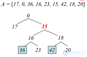
We will solve the RMQ problem, already knowing how to solve the LCA problem. To store the solution of the LCA problem we will use a treap (a Cartesian tree by implicit key). Then the minimum on the segment from i to j of the array A will equal the lowest common ancestor of the i-th and j-th elements in the treap built on the array A.
A treap by implicit key on the array A[1..N] — is a binary tree admitting the following recursive construction:
Here and below A[i] will also be used to denote the corresponding vertex of the tree.
Let's build a treap on the array AA. Then RMQ(i,j) = LCA(A[i],A[j]).
Let w=LCA(A[i],A[j]).
Note that A[i] and A[j] do not both belong simultaneously to either the right or the left subtree of w, because then the corresponding child would be located at a greater depth than ww, and would also be an ancestor of both A[i] and A[j], which contradicts the definition of LCA. From this remark it follows that w lies between A[i] and A[j] and, consequently, belongs to the segment A[i..j].
By construction we also know that:
Summarizing, we get that ww has the minimum value on the segment covering A[i..j], and belongs to the segment A[i..j], hence
RMQ(i,j)=w.
There exists an algorithm that builds a treap in O(n). Using the LCA construction algorithm, we get: preprocessing for LCA — O(n) and answering a query — O(1).
We need to build the treap once in O(n), perform preprocessing once in O(n), and answer queries in O(1).
As a result we get RMQ with construction in O(n) and query answering in O(1).

Comments