What are data structures and algorithms?
Data structures refer to the way data is organized and managed. Algorithms are predefined sequences of steps that can solve a problem efficiently.
Data structures and algorithms matter to every programmer. A deep knowledge of and skill with these two topics is the key to becoming a better professional and, ultimately, a higher-paid one.
Don't be afraid of math
Yes, data structures and algorithms involve some mathematical reasoning and proofs, especially when analyzing the time and space complexity of an algorithm.
But you don't need a high IQ or abstract mathematical knowledge. As long as you understand the basics of university-level math, you have the tools needed to understand data structures and algorithms.
This overview of data structures and algorithms lets you survey the most important subjects in computer science. You can grasp it quickly with the help of illustrations.
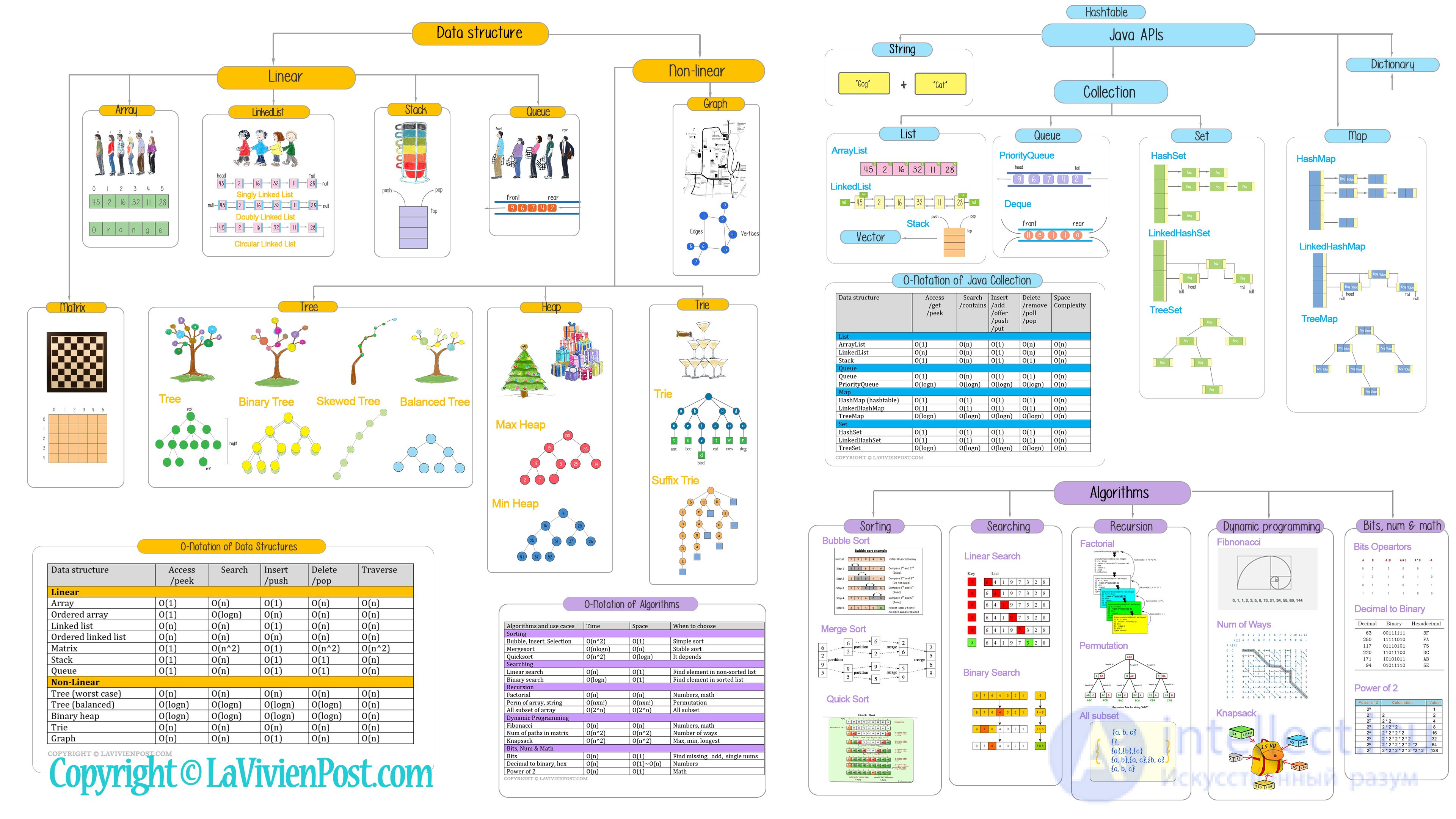
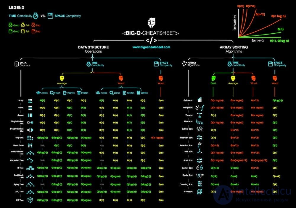
This lecture gives the big picture of data structures and algorithms
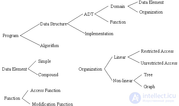
1 What are data structures?
Many definitions are available.
- A data structure is a collection of data components that together make up a meaningful whole.
- A data structure is a way of arranging data in computer memory or other disk storage.
- A data structure is a set of data organized in such a way that elements can be stored and retrieved by some fixed methods.
There are several common data structures: arrays, linked lists, queues, stacks, binary trees, hash tables, graphs, etc. These data structures can be classified as linear or nonlinear data structures, depending on how the data is conceptually organized or aggregated.
Linear structures. This category includes the array, list, queue and stack. Each is a collection that keeps its records in a linear sequence, and to which records can be added or removed as desired. They differ in the constraints they impose on how those records can be added, removed or accessed. Common constraints include FIFO and LIFO.
Nonlinear structures. Trees and graphs are classic nonlinear structures. Data records are arranged not in a sequence but according to various rules.
What are abstract data types (ADTs)?
Remember the goal of software engineering? Robustness, adaptability and reusability. From these efforts to write better code came a new metaphor for using and building data structures: the abstract data type, which emphasizes the notion of abstractness.
When we say "data type", we often refer to the primitive data types built into a language, such as integer, real, character and boolean. An integer is most likely implemented or represented in a computer by four bytes. However, when we use integers, we do not worry at all about their internal representation or how the compiler implements these operations in machine code. Moreover, we know that even when we run our program on a different computer, the behavior of an integer does not change, even though its internal representation may. What we know is that we can use primitive data types through their working interface: '+', '-', '*' and '/' for integers. Primitive data types were abstract entries.
A stack or a queue is an example of an ADT. Both stacks and queues can be implemented using an array. It is also possible to implement stacks and queues using linked lists. This demonstrates the "abstract" nature of stacks and queues: how they can be viewed separately from their implementation.
Applying the idea of abstraction to data structures gives us ADTs for data structures. On the one hand, an ADT clearly separates the interface from the implementation; the user sees only the interface and therefore must not interfere with the implementation. On the other hand, if the implementation of an ADT changes, the code that uses the ADT will not break, because the interface remains the same. Thus, abstraction makes code more robust and easier to maintain. Moreover, once an ADT is built, it can be used many times in different contexts. For example, a list ADT can be used directly in application code, or it can be used to build another ADT, such as a stack.
How do I choose the right data structures?
When writing a program, one of the first steps is to define or choose the data structures. What are the "right" data structures for a program? The interface of operations supported by a data structure is one of the factors to consider when choosing among several available data structures. Another important factor is the efficiency of the data structure: how much space does it take, and what is the running time of the operations in its interface?
2 What is an algorithm?
There are many definitions of algorithms. An algorithm is a procedure, a finite set of well-defined instructions for solving a problem, which, given an initial state, terminates in a defined end state. The computational complexity and efficient implementation of an algorithm are important in computing, and they depend on suitable data structures.
Classification of design techniques:
- Recursive
- Brute force
- Divide and conquer
- Depth-first
- Breadth-first
- Backtracking
- Greedy - locally optimal
- Branch and bound
Expressing an algorithm: there are many different ways to express an algorithm, including natural language, pseudocode, flowcharts and programming languages. Expressions of algorithms in natural language tend to be verbose and ambiguous, and are rarely used for complex or technical algorithms. Pseudocode and flowcharts are structured ways of expressing algorithms that avoid many of the ambiguities common to natural-language statements while remaining independent of a specific implementation language. Programming languages are primarily intended for expressing algorithms in a form that can be executed by a computer, but are often used as a way of defining or documenting algorithms.
Program efficiency: time vs. space. It is interesting to know how much of a given resource (such as time or storage) a given algorithm requires. Methods have been developed for analyzing algorithms to obtain such quantitative answers, such as big O notation. For example, the time needed to traverse an array of n slots is proportional to n, and we say the time is of order O ( n ). However, accessing the i-th element of an array takes only constant time, which does not depend on the size of the array, so it is of order O (1).
Definitions of running-time notation:
- Common functions used in analysis:
- Constant function f ( n ) = C - A constant algorithm does not depend on the input size.
- Logarithmic function f ( n ) = log n - the logarithmic function grows only slightly slower as n increases.
- Linear function f ( n ) = n - whenever n doubles, the running time increases.
- N-Log-N function f ( n ) = n log n - it grows slightly faster than the linear function.
- Quadratic function f ( n ) = n 2 - Every time n doubles, the running time increases fourfold.
- Cubic function and other polynomials
- Exponential function f ( n ) = b n
- Factorial function f ( n ) = n !
Classification of algorithms by asymptotic complexity
- O(1) – constant (checking whether a number is even or odd);
- O(n) – linear (find, search, etc.);
- O(logn) – logarithmic (binary search)
- O(nlogn) – quasilinear (Shell sort, quicksort)
- O(n 2 ) – quadratic
- O(2 n ) – exponential
Classification of algorithms by structure:
- Linear (sequence)
- Branching (branch, selection, alternative)
- Cyclic (repetition)
- Auxiliary
- Combined
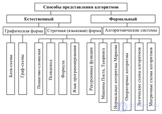
Fig. Classification of ways of representing algorithms
3. Data structures
With a data structure, we find ways to make access to data more efficient. When dealing with a data structure, we focus not just on a single piece of data but on various sets of data and how they can be related to each other in an organized way.
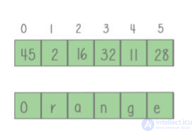
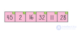
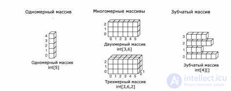
Array: an array is an index-based data structure, meaning each element is referenced by an index. An array contains elements of the same data type.
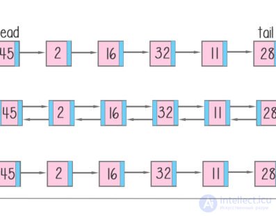
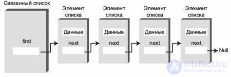
Linked list: a linked list is a sequence of nodes in which each node is linked to the node that follows it. This forms a link in a chain of data storage. It consists of data elements and a reference to the next record.
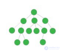
Tree: a tree is a set of nodes connected by edges. Each node points to several nodes. A tree is a hierarchical graphical form.
Binary tree: a binary tree has 1 or 2 child nodes. It can have as few as zero nodes, which happens when the nodes have NULL values.
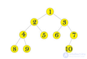
Binary search tree: a binary search tree (BST) is a binary tree. The left subtree contains nodes whose keys are less than the node's key value, and the right subtree contains nodes whose keys are greater than or equal to the node's key value. Moreover, both subtrees are also binary search trees. A binary search tree can retrieve data efficiently.
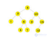
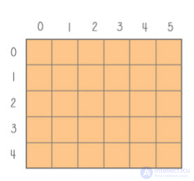
Matrix: a matrix is a two-dimensional array. It uses two indices, row and column, to store data.
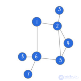
Graph: a graph contains a set of nodes and edges. Nodes are also called vertices. Edges are used to connect nodes. Nodes are used to store and retrieve data.
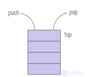
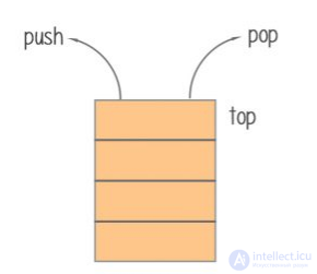
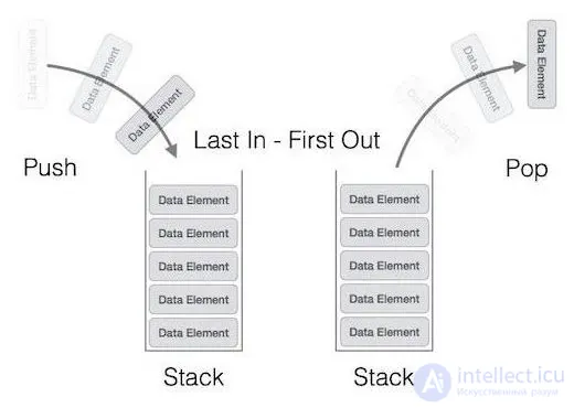
Stack: a stack is a LIFO data structure in which only the top element is accessible. Data is added by pushing and removed by popping from the top.
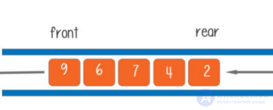
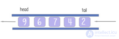
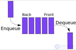
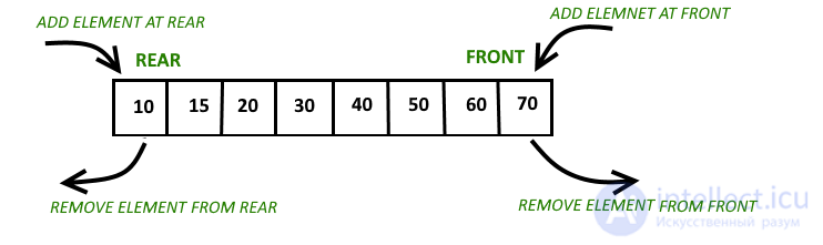
Queue: a queue is a FIFO data structure. In this structure, new elements are inserted at one end and existing elements are removed from the other.
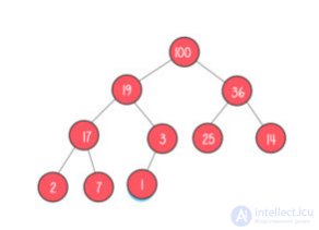
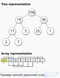
Max-Heap: a heap is a tree-based data structure in which all the nodes of the tree are arranged in a specific order. A max-heap is a binary tree. It is complete. The data element stored in each node is greater than or equal to the data elements stored in its child nodes.
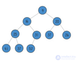
Min-Heap: a min-heap is a binary tree. It is complete. The data stored in each node is less than the data elements stored in its child nodes.
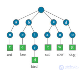
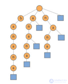
Trie: A trie - is a tree. In a trie, each node (except the root) stores a single character or digit. By traversing the trie down from the root node to a particular node n, a common prefix of characters or digits can be formed, which is also shared by other branches of the trie.
Suffix tree: a suffix tree is a tree containing all the suffixes of a given text. A suffix tree makes many important string operations especially fast to implement.
4. Java Collections
The Java Collections Framework is a set of collection types included as part of core Java. It provides APIs, or methods, that you can use directly to work with data structures such as arrays, linked lists, stacks, queues, sets and maps. If you master Java collections, it will save you a lot of time and help you solve complex problems.
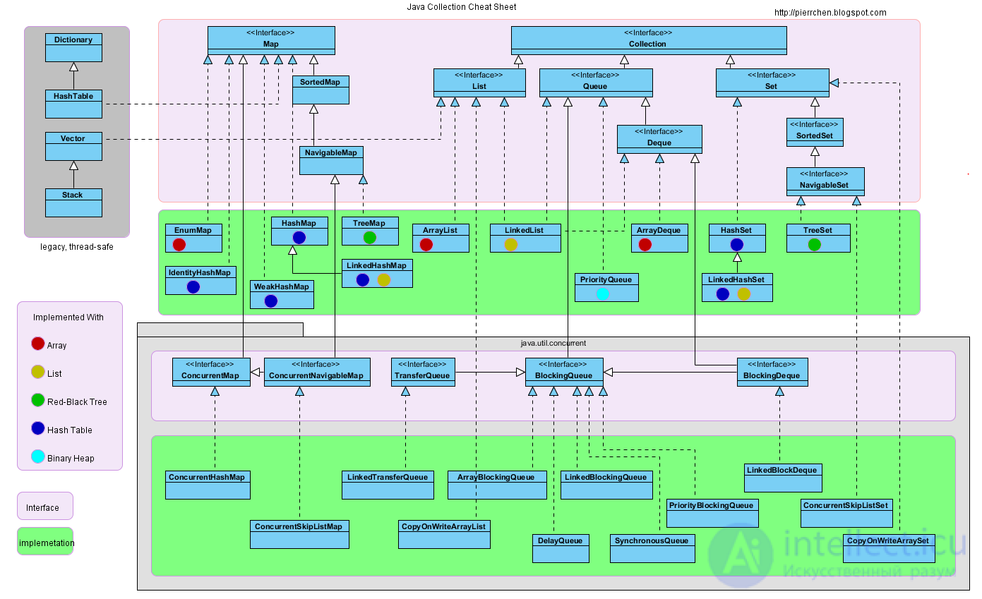
ArrayList: the ArrayList class is a resizable-array implementation of the List interface. It implements all optional list operations and permits all elements.
Vector: Vector is very similar to ArrayList, but Vector is synchronized and slow. It is a legacy class and is now compatible with collections.
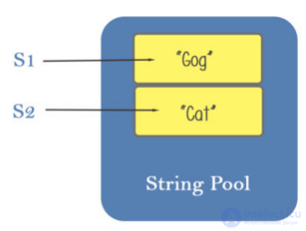
String: the String class is used to create and manipulate strings.
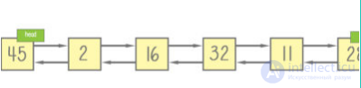
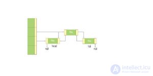
LinkedList: the LinkedList class is a doubly-linked list implementation of the List and Deque interfaces. LinkedList stores its data as a list of elements, and each element is linked to its previous and next element.
HashMap: HashMap is a collection class that implements the Map interface. It requires a hash function and uses the hashCode() and equals() methods to put elements into and retrieve them from the collection, respectively.
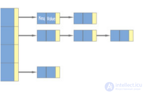
Hashtable: the Hashtable class is similar to HashMap. It implements a dictionary. Hashtable provides an enumeration of its keys. It does not allow null as a key or value. Note that because HashMap was created later, it is an enhanced version and improvement of Hashtable. Hashtable is synchronized and slower. HashMap is preferred over Hashtable.
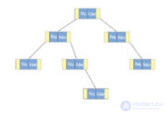
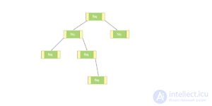
TreeMap: TreeMap implements the SortedMap interface. It is sorted in ascending order of keys. The complexity of operations is O(logn).
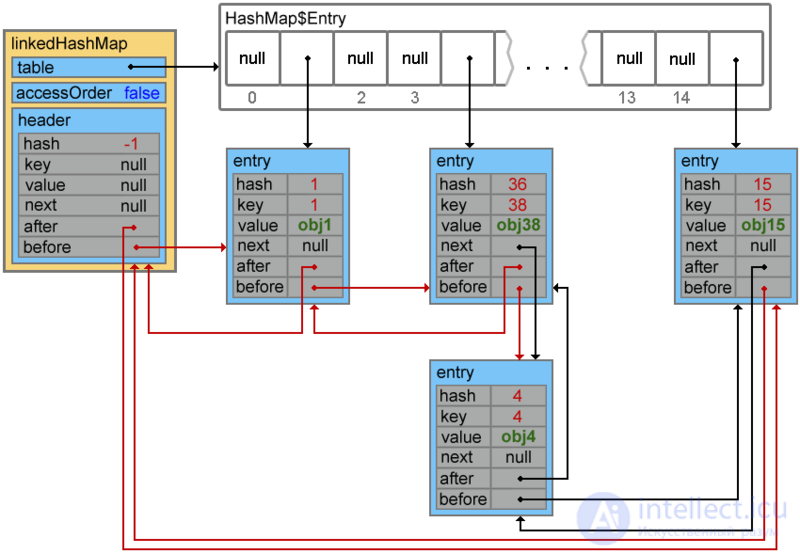
LinkedHashMap: LinkedHashMap preserves insertion order. The complexity is the same as HashMap, O(1).
HashSet: the HashSet class implements the Set interface. Duplicate values are not allowed. Its elements are unordered. NULL elements are allowed in a HashSet.
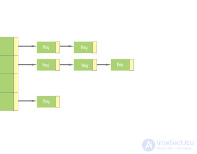
TreeSet: TreeSet is implemented using a tree structure. Elements in a TreeSet are sorted. The complexity of operations is O(logn).
LinkedHashSet: LinkedHashSet maintains insertion order. Elements are ordered in the same sequence in which they were added to the set. The complexity is the same as HashSet, O(1).
Stack: the Stack class extends the Vector class with five operations to support LIFO (Last In First Out). Inside the stack there is a pointer, TOP, which points to the top element of the stack.
PriorityQueue: the PriorityQueue class is an implementation of Queue in which each element has an associated priority. The elements of a priority queue are ordered according to their natural ordering or by a comparator provided at queue construction time.
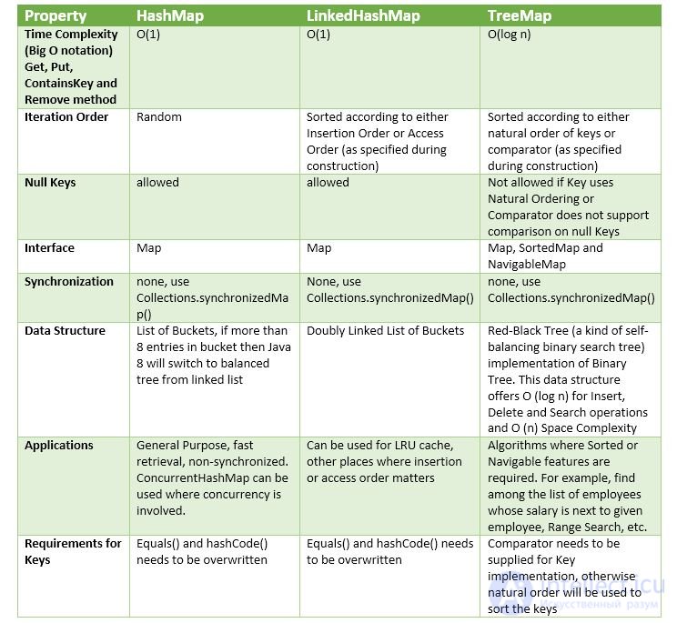
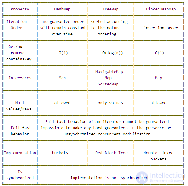
Difference between HashMap, LinkedHashMap and TreeMap
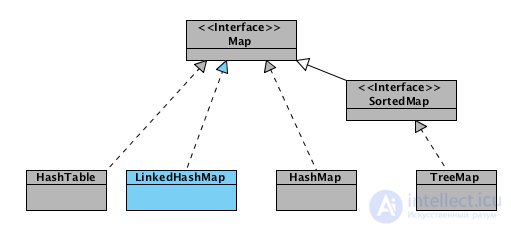
All three classes implement the Map interface and offer mostly the same functionality. The most important difference is the order in which iteration over the entries will occur:
HashMap
- gives absolutely no guarantees about iteration order. The order may (and will) even change completely when new elements are added.
- It holds paired values (key, value)
- NO duplicate keys
- unordered and unsorted
- it allows one null key and more than one null value
TreeMap
- iterates in the "natural ordering" of the keys according to their
compareTo() method (or an externally supplied Comparator ). In addition, it implements the SortedMap interface, which contains methods that depend on this sort order.
- The ordered and sorted version
- based on hashing data structures
LinkedHashMap
- iterates in the order in which the entries were put into the map
- This is the ordered version of the Map implementation
- Based on a linked list and hashing data structures
HashTable
- the same as a hash map
- it does not allow a null key or null values
"Hashtable" is the generic name for hash-based maps. In the context of the Java API, Hashtable is an obsolete class dating from Java 1.1, before the collections framework appeared. It should no longer be used, because its API is cluttered with obsolete methods that duplicate functionality, and its methods are synchronized (which can reduce performance and is generally useless). Use ConcurrentHashMap instead of Hashtable.
5. Algorithms
An algorithm is a well-defined procedure that allows a computer to solve a problem. There are many algorithms. Here I list several widely used algorithms in computer science: sorting, searching, recursive programming, and dynamic programming.
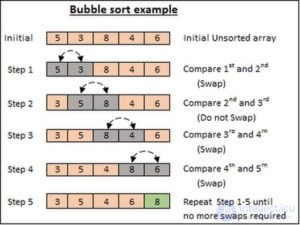
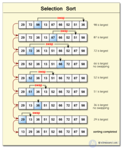
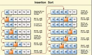
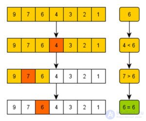
Sorting: Sorting is an algorithm consisting of a series of instructions that take an array as input, perform certain operations on the array, sometimes called a list, and output a sorted array. Simple sorting algorithms are bubble sort , selection sort , and insertion sort .
Bubble sort: this is the simplest sorting algorithm. We start at the beginning of the array and swap the first two elements if the first is greater than the second. Then we move on to the next pair and so on, continually passing through the array until it is sorted. O(n 2) average and worst case.
Selection sort: this is the most intuitive, though not necessarily efficient. Find the smallest element using a linear scan and move it to the front (by swapping it with the front elements). Then find the second smallest and move it, again performing a linear scan. Keep doing this until all the elements are in place. Suitable for small files. O(n 2) average and worst case.
Insertion sort: sorts an array by shifting elements one by one. Each iteration removes an element from the input data and inserts it into the correct position in the list being sorted. It is efficient for small data sets but very inefficient for large lists. It is better than selection sort and bubble sort. O(n 2) average and worst case.
Searching: searching consists of finding content based on a key. There are linear search and binary search .
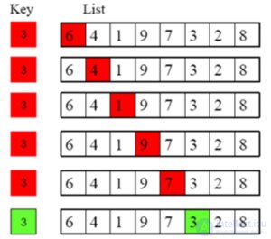
Linear search: linear search is a method of finding a target value in a list. It sequentially checks each element of the list against the target value until a match is found or until all the elements have been checked.
Binary search: binary search is an efficient algorithm for finding an element in an ordered list of elements. It works by repeatedly halving the part of the list that could contain the element, until you have narrowed the possible locations down to one. The complexity is reduced from O(n) to O(logn).
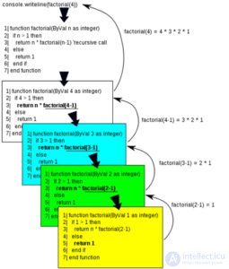
Recursion: recursion is a computer programming technique in which a function or algorithm calls itself. It must include a step with a termination condition. When the condition is met, the rest of each repetition is processed from the last call back to the first. The best-known problem solved with recursion is the Factorial .
Factorial: The factorial of a number n is the product of all positive nonzero integers less than or equal to n. The factorial of n is denoted n !.
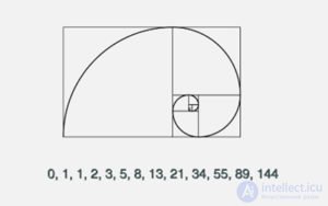
Dynamic programming: dynamic programming is a method of solving a complex problem by breaking it down into a set of simpler subproblems, solving each of these subproblems only once, and storing their solutions. The next time the same subproblem occurs, the previously computed solution is looked up, thereby saving computation time at the expense of a modest amount of storage space. A famous dynamic programming problem is the Fibonacci numbers .
Fibonacci numbers: this is a sequence of numbers in which each number (a Fibonacci number) is the sum of the two preceding numbers. The simplest is the sequence 1, 1, 2, 3, 5, 8, etc.
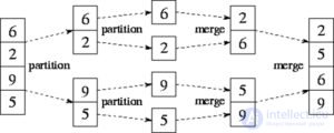
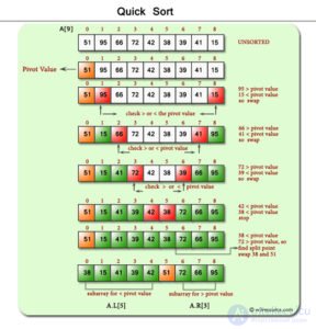
Divide and conquer: a divide-and-conquer algorithm works by recursively breaking a problem down into two or more subproblems of the same or a related type until they become simple enough to be solved directly. Well-known divide-and-conquer problems are merge sort and quicksort .
Merge sort: divides the array in half, sorts each of these halves, and then merges them together. The same sorting algorithm is applied to each of these halves. In the end, it merges two single-element arrays. O(nlogn) average and worst case.
Quicksort: picks a random element and partitions the array so that all numbers smaller than the partitioning element come before all elements greater than it. If we partition the array around an element several times, the array will eventually become sorted. But because the partitioning element is not guaranteed to be the median, our sort can be very slow. O(nlogn) on average, O(n 2) in the worst case.
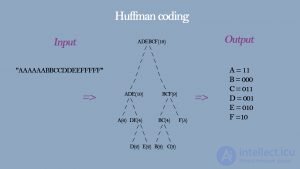
Greedy : A greedy algorithm makes the choice that seems best at the moment, i.e., it makes a locally optimal choice in the hope that this choice will lead to a globally optimal solution. A well-known problem solved by greedy algorithms is Huffman coding .
Huffman coding: Huffman coding is a lossless data compression algorithm. The idea is to assign variable-length codes to the input characters, where the length of each assigned code is based on the frequency of the corresponding character.
Comparison table of the main data structures:
| Characteristic |
Queue |
Stack |
Linked List |
Array |
Deque |
Heap |
|
Principle of operation

|
FIFO (first in, first out) |
LIFO (last in, first out) |
Elements are linked by pointers |
Indices are fixed |
Access to both ends |
A tree where the parent is >= (max heap) or <= (min heap) its children |
|
Adding elements

|
At the end (enqueue) |
At the end (push) |
At the beginning or end |
At any position |
At the beginning or end |
At the root (with rebalancing) |
|
Removing elements

|
From the beginning (dequeue) |
From the end (pop) |
At any position (requires traversal) |
At any position (but requires shifting) |
At the beginning and end |
From the root (with reordering) |
|
Accessing elements

|
Only the first (head) |
Only the last (top) |
Sequential (via references) |
Direct access by index |
At the beginning and end |
Only the root (the largest or smallest element) |
|
Running time (average)

|
O(1) (add/remove) |
O(1) (add/remove) |
O(1) (add at the beginning/end) |
O(1) (access), O(n) (insert/remove) |
O(1) (operations at the ends) |
O(log n) (add, remove, access the root) |
| Where it is used |
Background tasks, thread management, BFS algorithms |
Recursion, undoing actions (Ctrl+Z) |
Dynamic structures, graph traversal |
Static structures, fast access |
Buffers, parsers, data processing |
Priority queue, Dijkstra's and Huffman algorithms, storing classes |
| |
 |
 |
 |
 |
 |
 |
See also
- [[b4474]]
- [[b4476]]
- [[b4477]]
- [[b7729]]
- [[b4478]]
- [[b4404]]
- [[b9580]]
- [[b3952]]
- [[b3953]]
- [[b12935]]
See also


Comments